Model Tracking and Accuracy Analysis | Deep Learning

Without performance analysis, anyone can’t grow his activities. In deep learning, model tracking, and accuracy analysis are the key points for assuring the best model and development. Deep learning is a field of experiments. A practitioner needs to experiment more with a problem to get the best model. To understand which is the best model for a problem, we have to understand the model tracking and accuracy analysis objectives deeply. Today we will discuss this topic and give you an overall idea. Let’s get started.

Before jumping into the details of the tutorials, let’s know about the subtopics of the tutorial are given below.

• Introduction

• Model Tracking 

• Accuracy Analysis

• Monitoring Model Performance

• Model Interpretability and Explainability

• Accuracy Improvement Strategies

• Challenges and Considerations

• Conclusion

Introduction

Model tracking and accuracy analysis are critical steps in the deep learning lifecycle. Model tracking indicates the process of recording and tracking various objectives of the model over time. We generally experiment on different versions of models, use different hyperparameters, and see the performance of the model by performance metrics such as accuracy, F1 score, dice score, and so on for both training and validation datasets. For each experiment with a definite model and hyperparameters, we can keep a record of the performance of the model and then we can choose the best model and hyperparameters for the problem. We can also experiment on layers of the model and features of the dataset which are responsible for creating the best model by model tracking.

Accuracy analysis indicates the performance of the deep learning model. To understand how much a model can perform for both training and validation datasets, accuracy analysis plays an important role. There are various types of performance metrics to analyze the accuracy of the model such as accuracy, AUC-ROC, precision, recall, MAE, MSE, RMSE, and so on.

You can see the details in the following tutorials. Now let’s understand the importance of using model tracking and accuracy analysis in the model given below.

• Understanding the model performance by tracking models and analyzing their performance.

• Model tracking allows us to record the effects of hyperparameters on model performance and can find the best combinations.

• We can detect the overfitting problem.

• We can interpret and explain the model.

• If the model started to overfit, we can stop the training process by tracking and accuracy analysis.

There are many other benefits of model tracking and accuracy analysis for getting a more robust and better model. Overall, Model tracking and accuracy analysis are essential in building, selecting, and maintaining effective models in deep learning. 

Model Tracking 

Model tracking refers to the practice of systematically recording and monitoring information about the models during the training and development process. Model tracking can be used to record the performance of the model’s architecture, hyperparameters, training and validation metrics, performance on test data, or any change or updates made to the model over time. It is essential for evaluating, comparing, optimizing, and managing models in the project.

You can track the model for various perspectives that are given below.

• By changing the number or type of the layers in the Model Architecture over time, you can track the model and choose the best model architecture for your problem domain.

• You can experiment on hyperparameters(such as learning rate, batch size, number of epochs and so on) over time and can choose the best one. 

• You can experiment on training and validation data such as the number of samples, features used or various data processing steps and can track the performance over time. 

• You can experiment with various metrics and track the performance and choose the best model.

The main thing in model tracking is recording and analyzing the experiments of the models in various ways. Hope, you can understand in which ways, we can use model tracking in deep learning. Now let’s learn about the benefits of using model tracking in the deep learning lifecycle.

• We can compare different models or different versions of the same model for a problem domain. Then we can choose the best model for deployment.

• We can monitor the performance over time which will give us a better understanding of how a model is learning and how changes to hyperparameters or model architecture can impact performance. 

• Model tracking records all parameters, hyperparameters, and other sources that can be used to reproduce the model precisely.

• As a teamwork, multiple practitioners can see what types of attempts have already been done and the results also by model tracking that reduces duplicate work and improves efficiency.

• If a model fails and gives unexpected errors. Then by tracking we can diagnose what goes wrong on the model. 

Overall, model tracking helps you to find the best model for deploying your problem and also helps to overcome many problems that occur in the model.

Tools and Techniques for Model Tracking

To do model tracking efficiently, a number of tools have been developed over time with different facilities. Today we will gather some knowledge about some tools that are popular and widely used in the developers community. Let’s start.

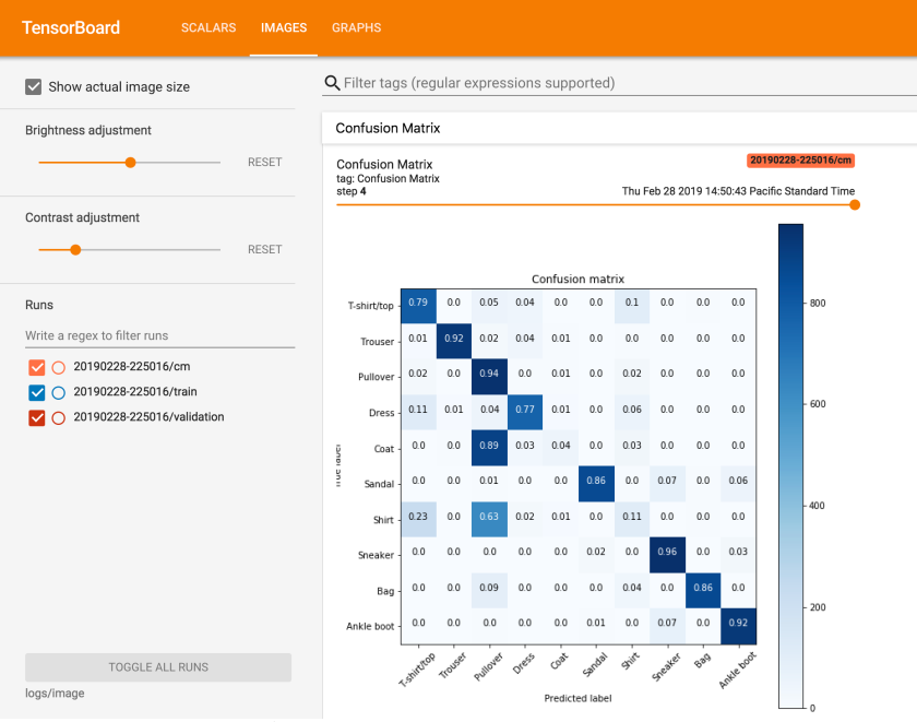
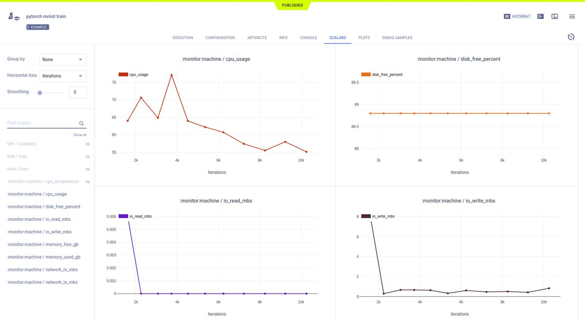
• Tensorboard: It is a visualization toolkit that allows visualization of metrics such as training and validation loss, accuracy, and so on. You can visualize the model architecture, embeddings, and even image or audio data. This tool is very useful for tracking the model during training and understanding the model performance with different experiments.

  

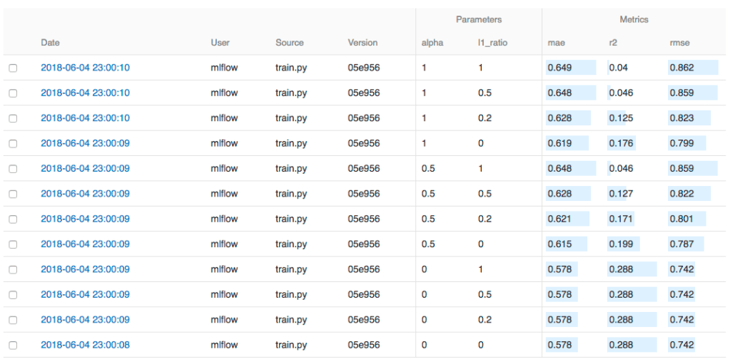
• MLFlow: It is an open-source platform for managing the end-to-end machine learning lifecycle. This tool is used for tracking experiments, packaging code into reproducible runs, sharing models, deploying models, and so on. This tool has mainly four components such as MLflow tracking, MLflow projects, MLflow models, and MLflow Registry. MLflow tracking is used for tracking experiments to record and compare the results and parameters of the model. MLflow projects provide a standard format for packaging reusable code and you can launch any MLflow project from Git URL. MLflow models allow you to manage and deploy models from a variety of ML libraries. MLflow registry is a centralized model store, set of APIs, and UI that manage the full lifecycle of an MLflow model.

  

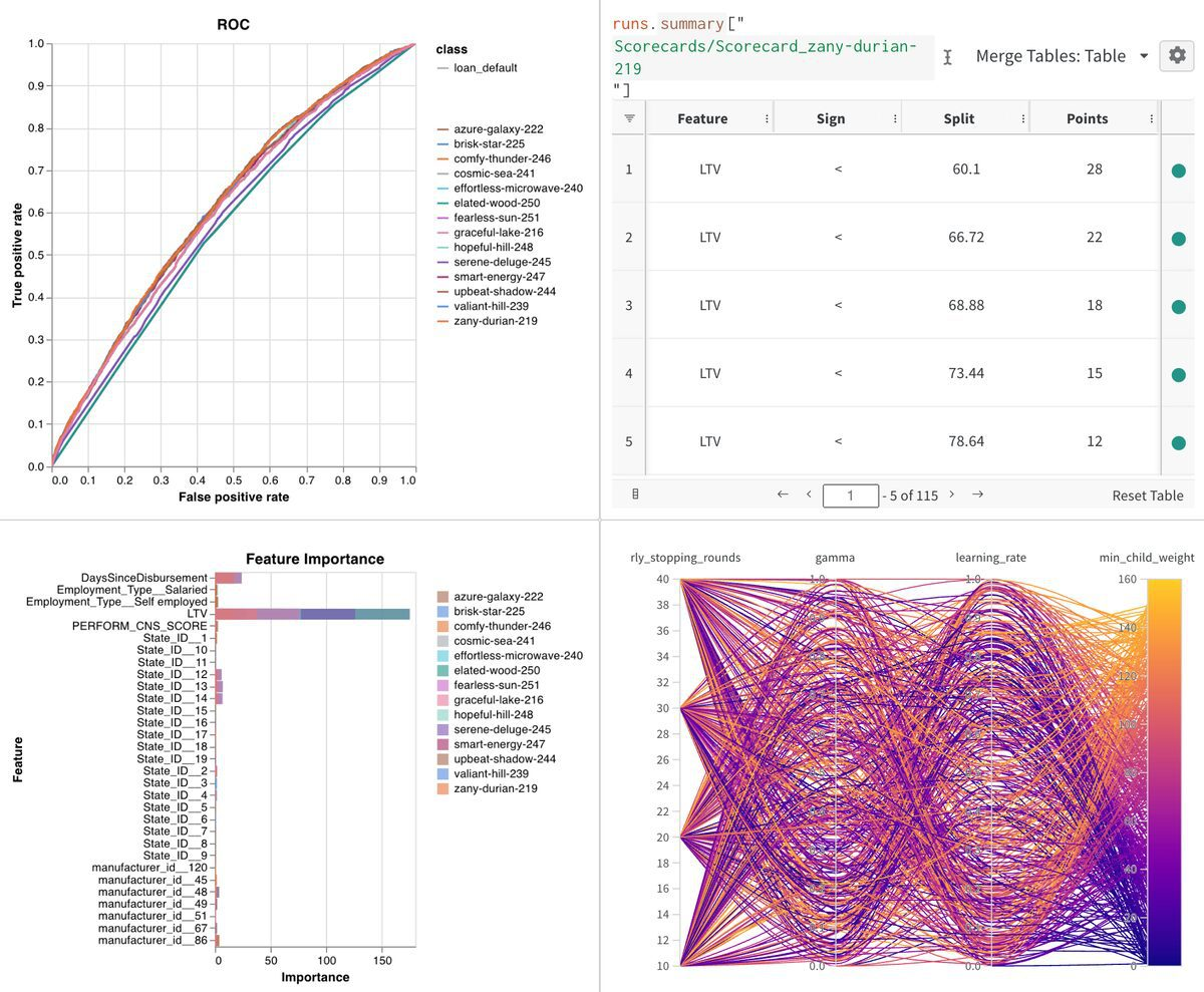
• Weight & Biases (wandb): It is used for experiment tracking, dataset versioning, and model management. You can visualize and compare the results of your model in a centralized, interactive dashboard. The key components of Weight and Biases are experiment tracking of your model (logging all aspects of your machine learning runs such as hyperparameters, metrics, model architectures, and so on), a rich set of visualization tools, collaboration(share your results with your colleagues), integration a number of popular deep learning libraries, model management, artifacts tracking, reproducibility and so on. 

  

• Neptune.ai: It is a rich toolkit for model tracking and model management. The features of Neptune are tracking and logging all aspects of your machine learning experiments(including hyperparameter, model architecture, and so on), Notebook integration(integrate jupyter notebook in Neptune UI), Model management, data versioning, collaboration and sharing your experiments and results, comparison and analysis, popular machine learning libraries integration, Notification, reports and so on. Also, it is designed to be lightweight and flexible.

  

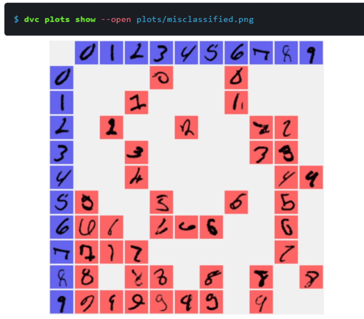
• DVC (Data Version Control): It is an open-source version control system that is designed to handle large files, datasets, machine learning models, and metrics as well as code. It provides full reproducibility and collaboration in machine learning workflows. The features of DVC are Data Versioning(handling large files of data as well as keeping track of changes in your data), Model Versioning(keeping track of different versions of models), Reproducibility, Pipeline Management(managing the stage of ML workflow), Experiment Management(compare multiple experiments), Data transfer(integrates various storage platforms like local drive, S3, azure and so on), and Metrics Tracking. It is a command line tool that integrates well with jupyter notebooks, machine learning libraries, and cloud services. It is also a lightweight and flexible tool.

  

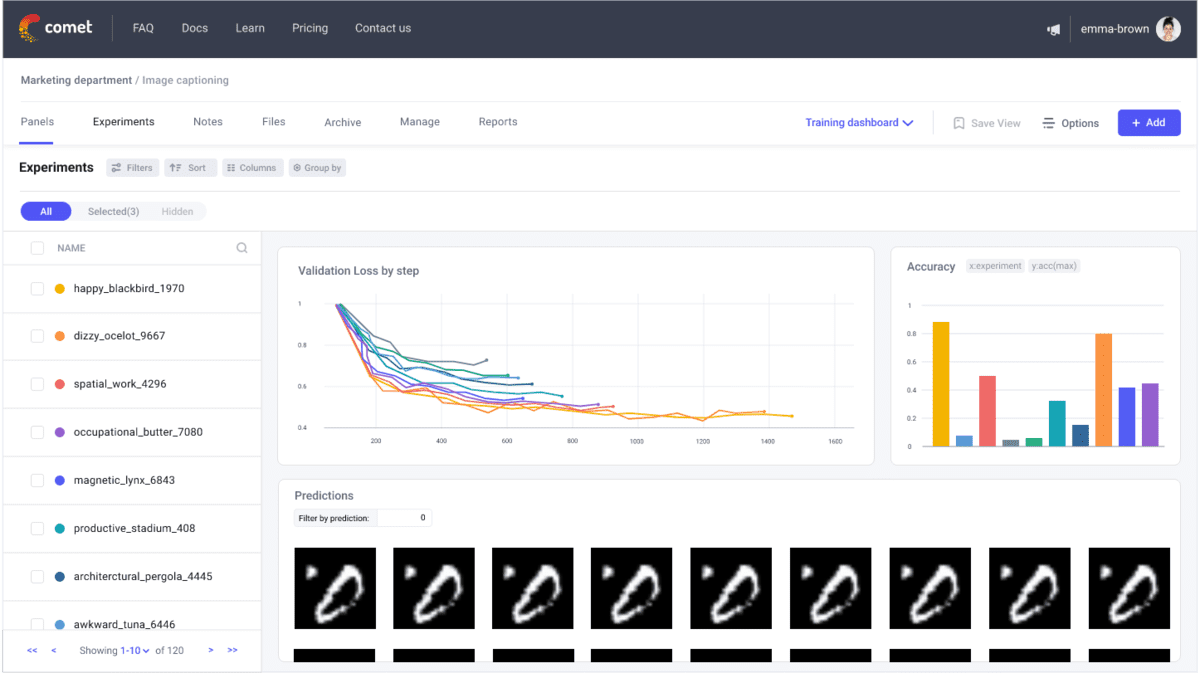
• Comet.ml: It is a machine-learning platform that allows you to automatically track, compare, explain, and reproduce machine-learning experiments. The features of Comet are Experiment tracking, visualization, Code versioning, Model Management, integration, collaboration and sharing the results with others, Hyperparameter optimization, Interpretability, notification, and others. Practitioners can focus more on model development and experimentation.

  

• ClearML: It is an open-source Machine Learning Operations(MLOps) platform that is designed to automate preparing, executing, and analyzing machine learning experiments. It is used to manage the machine learning lifecycle. The features of ClearML are Experiment tracking, Model management, Integration, Collaboration, Pipeline management, Automatic Resource Management, Data Management, and deployment. It is flexible and adaptable fitting into any machine learning workflow, from single-user to large-scale enterprise environments.

  

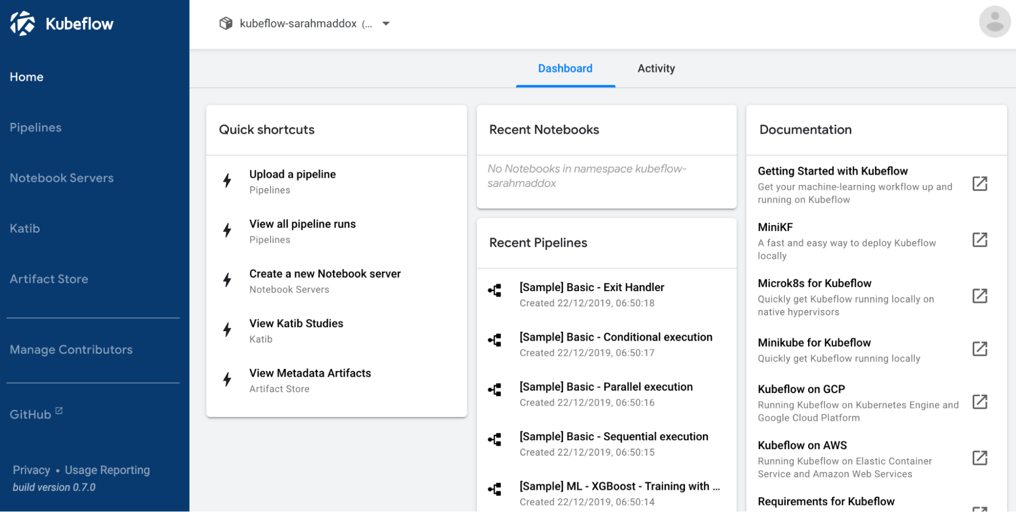
• Kubeflow: It is an open-source project that provides ML tools in Kubernetes. It makes ML workflows on Kubernetes simple, portable, and scalable. Kubeflow can be integrated with other tools such as MLflow, Tensorboard, and others for model tracking. The features of Kubeflow are kubeflow pipelines for end-to-end ML workflow, katib for hyperparameter tuning, KFServing for ML frameworks, Integration with machine learning libraries, Portability, scalability, Multi-user support, and so on. 

  

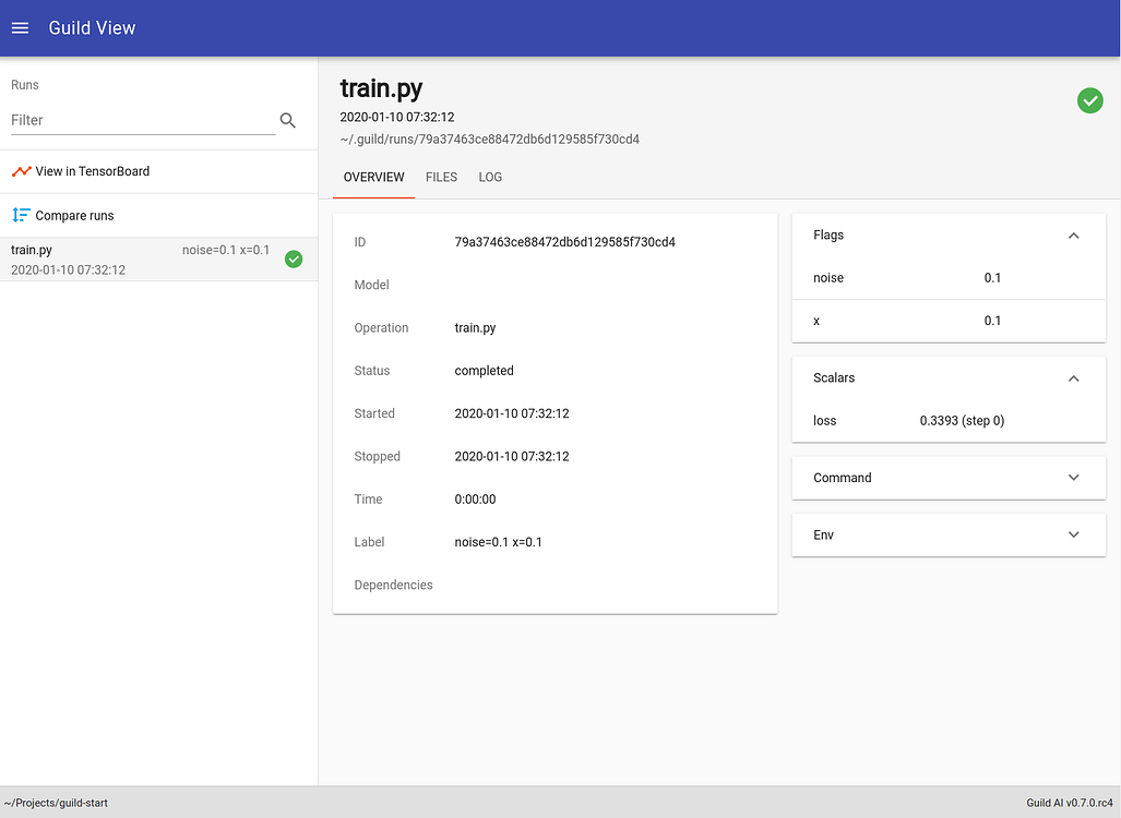
• Guild.ai: It is also an open tool that is used to manage and experiment with machine learning models. The features of Guild AI are Experiment Tracking, Automation, Version control, Resource management, Integration, Privacy, Ease of use, and visualization. Generally, it makes machine learning development more efficient.

  

There are other tools for model tracking such as Polyaxon, Scared, Omniboard, Valohai, Pachydarm, Verta.ai, Sagemaker studio, Optuna and so on. Maybe in other tutorials, we will discuss those model-tracking tools. Hope, you can understand the concept of model tracking, benefits, and tools in this field. Now we will move to the accuracy metrics that are used to measure the performance of the model. 

Accuracy Analysis

Accuracy analysis indicates the process of evaluating how well the model has learned from the training data and can generalize to unseen data. It is a quantitative measure of how closely the model’s predictions match the actual or true values. With the help of accuracy analysis, we compare the different models and select the best one for a particular task. 

Benefits of Accuracy Analysis

Actually, it is the core concept of Deep Learning. It has several benefits that are given below.

• It gives a clear understanding of how well the model is performing. 

• We can compare different models with the help of accuracy analysis.

• It gives an idea to choose the best hyper-parameters for the model.

• We can detect the model condition such as overfitting, underfitting, or appropriate fitting, and can take necessary steps for further work.

• Different performance metrics capture different aspects of the model’s performance such as precision measures of how many of the positive predictions are correct and recall measures of how many actual positives are identified. So having multiple metrics gives you an understanding of these trade-offs and makes informed decisions. 

• It provides a baseline from which to improve.

• We can communicate the model’s performance to the stakeholders in a clear quantitative way.

Evaluation Metrics 

The choice of the evaluation metric depends on the task at hand. The problem can be classification, regression, or others. The aspects of the problem can vary. So, a number of evaluation metrics have been developed for specific tasks. Some details of evaluation metrics are given below.

• Accuracy: It is used in classification problems that give a ratio of correct prediction to the total number of predictions. 

  Accuracy = (Number of correct predictions) / (Total number of predictions)

  It is simple but it has limitations such as it can’t give a good overview of an imbalanced dataset and it treats all errors are equal.

• Precision: It is used in classification problem that gives a ratio of true positive predictions to all positive predictions. It measures how many of the positively classified predictions are actually correct.

  Precision = True Positives / (True Positives + False Positives)

  It is a useful metric but might not be very informative when the positive class is rare.

• Recall: It is also used in classification problem that gives a ratio of true positive predictions to all actual positive instances. It provides a measure of the model’s ability to correctly identify positive instances out of all actual positive instances.

  Recall = True Positives / (True Positives + False Negatives)

  A high recall means the model correctly identifies a large proportion of positive instances. Precision, Recall metrics are very much important in medical image prediction. 

• F1-score: It is the harmonic mean of Precision and Recall. It provides a balance between precision and recall.

  F1 Score = 2 * (Precision * Recall) / (Precision + Recall)

  The range of the F1 score is 0 to 1. 1 indicates the perfect precision and recall, and 0 indicates either precision is zero or recall. F1 score assumes that precision and recall are equally important.

• Area Under the ROC Curve(AUC ROC): The area under the Receiver Operating Characteristics curve is a performance metric that is used in Machine learning and Deep Learning for binary classification. It can also extend into multiclass classification. The ROC curve is a plot that displays the performance of a binary classifier. The plot is the True Positive Rate(TPR) against False Positive Rate(FPR).

  True Positive Rate (Recall) = True Positives / (True Positives + False Negatives)
  False Positive Rate = False Positives / (False Positives + True Negatives)

  The AUC ROC is the area under the ROC curve that provides an aggregate measure of performance across all possible classification thresholds.

Implementation of Classification Metrics

You will get the code in Google Colab also.

from sklearn.metrics import accuracy_score, precision_score, recall_score, f1_score, roc_auc_score
y_true = [0, 1, 1, 0, 1, 0, 1, 0, 0, 1]
y_pred = [0, 0, 1, 0, 1, 0, 1, 1, 0, 1]
accuracy = accuracy_score(y_true, y_pred)
print("Accuracy:", accuracy)
precision = precision_score(y_true, y_pred)
print("Precision:", precision)
recall = recall_score(y_true, y_pred)
print("Recall:", recall)
f1 = f1_score(y_true, y_pred)
print("F1 Score:", f1)
# for roc auc, y_score are the predicted probabilities
y_true = [0, 1, 1, 0, 1, 0, 1, 0, 0, 1]
y_score = [0.1, 0.3, 0.8, 0.2, 0.6, 0.1, 0.9, 0.5, 0.3, 0.7]
auc_roc = roc_auc_score(y_true, y_score)
print("AUC-ROC:", auc_roc)

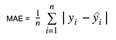
• Mean Absolute Error(MAE): This metric is used for regression tasks that indicate the average of the absolute differences between the predicted and actual values.

  It is the average of the absolute differences between the prediction and the actual observation. It is less sensitive to outliers. 

• Mean Squared Error(MSE): Like MAE, it is also a regression task that measures the average of the squared difference between the actual values and predicted values.

  

  It gives large errors compared to MAE. It is more sensitive to Outliers than Mean Absolute Error(MAE). 

• Root Mean Squared Error(RMSE): RMSE is the square root of Mean Square Error(MSE). Because of the Square Root of MSE, RMSE gives a sense of how much error the model typically makes in its predictions.

  

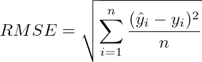
  RMSE is easier to interpret the results than MSE. 

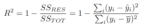
• R-Squared: It is known as the coefficient of determination that is used in a regression problem. It provides a measure of how well-observed outcomes are replicated by the model, based on the proportion of total variation of outcomes explained by the model.

  

Implementation of regression metrics

from sklearn.metrics import r2_score,mean_squared_error, mean_absolute_error
y_true = [1, 2, 3]
y_pred = [1, 2, 3.1]
mae = mean_absolute_error(y_true, y_pred)
print("Mean Absolute Error (MAE):", mae)

mse = mean_squared_error(y_true, y_pred)
print("Mean Squared Error (MSE):", mse)

rmse = np.sqrt(mean_squared_error(y_true, y_pred))
print("Root Mean Squared Error (RMSE):", rmse)

r2 = r2_score(y_true, y_pred)
print(“R squared:”, r2)

Holdout Validation and Cross-Validation

These two methods are used to access the performance of the machine learning model. They estimate how effective the model is likely to be in practice and can be used to prevent the overfitting problem. 

In Holdout validation, the dataset is split into two parts(training and testing dataset). The model is trained on a training dataset and for evaluating the model performance, the testing dataset is used. The ratio of training and testing datasets can be 80%: 20% or 70%: 30% or others. It is simple and computationally efficient.

Holdout Validation Implementation

from sklearn.model_selection import train_test_split
#develop a model and other utilities 
—-------------------
model.fit(X_train, y_train, epochs=10, batch_size=32)
# Evaluate the model
scores = model.evaluate(X_test, y_test, verbose=0)
print("Holdout Validation Accuracy: %.2f%%" % (scores[1]*100))

In the Cross-validation, it solves some of the issues of holdout validation. Here the data is split into k equally sized subsets or folds. The model is trained and tested in k times, each time the model trained on k-1 folds and tested on the remaining fold. The performance of the model is then averaged over the k trials to provide an overall performance of the model. It provides a more robust model performance than holdout validation because it uses the entire dataset for both training and testing. Because of taking a number of times training and testing, cross-validation is more computationally expensive than Holdout validation.

Cross Validation Implementation

from keras.wrappers.scikit_learn import KerasClassifier
from sklearn.model_selection import cross_val_score, KFold
# make a model & Wrap our Keras model in an estimator compatible with scikit_learn
estimator = KerasClassifier(build_fn=create_model, epochs=10, batch_size=32, verbose=0)
# use scikit_learn's cross_val_score to do cross validation
kfold = KFold(n_splits=5, shuffle=True, random_state=42)
results = cross_val_score(estimator, X, y, cv=kfold)
print("Cross Validation Accuracy: %.2f%% (%.2f%%)" % (results.mean()*100, results.std()*100))

Confusion Metrics and Classification reports

These are important tools to analyze the performance of the classification model. They provide different views of how well the model is performing.

A confusion Matrix is a table layout that gives a visualization of the performance of the classification problem. It has two dimensions (actual/expected, predicted). Each dimension has as many categories as there are in the target variable. In the below graph, there are four categories in the target variable. So the dimension is 4*4. Where the green boxes indicate the predicted value and actual value are the same. Pink boxes indicate the wrong prediction.

A classification report is a display of precision, recall, f1-score and support for each category in a classification problem. It gives more details of the performance for each class. Here precision, recall, f1-score are discussed above. Support is the number of actual occurrences of the class in the dataset.

Implementation in python

from sklearn.metrics import confusion_matrix, classification_report
y_true = [0, 1, 0, 1, 1, 0, 1, 0, 0, 1]
y_pred = [0, 0, 1, 1, 1, 0, 1, 1, 0, 0]
print("Confusion Matrix:")
print(confusion_matrix(y_true, y_pred))
print("Classification Report:")
print(classification_report(y_true, y_pred))

Residual Analysis for the regression model

It is a fundamental step in the regression model evaluation process. The residuals of a model are the differences between the actual and predicted values. Easily they are the errors of the prediction values. It is used to validate the assumption of the regression model and check whether the errors are random or not. If the errors are not random, then the model can be improved by other activities. You can understand whether the condition of the errors is random or not by the residual plot.

Implement the residual plot

import matplotlib.pyplot as plt
import seaborn as sns
residuals = [e1-e2 if e1>e2 else e1 for (e1, e2) in zip(y_true ,y_pred)]sns.residplot(x=y_pred, y=residuals, lowess=True, color="g")
plt.xlabel('Fitted values')
plt.ylabel('Residuals')
plt.title('Residual Plot')
plt.show()

Monitoring Model Performance

Monitoring model performance is a crucial step for machine learning system maintenance. It allows you to detect and rectify any deterioration in the model’s performance due to factors such as concept drift, changing data distribution, or evolving real-world scenarios. There are several ways to monitor the model performance such as continuous evaluation, real-time monitoring, Performance metrics tracking, Concept Drift Detection, set thresholds to perform alerts and triggers, residual analysis, Error analysis, A/B testing, and so on. Let’s go deep about the topics. 

Continuous monitoring: It is crucial for maintaining its effectiveness over time. As new data comes in, the assumptions of the model were originally built on might no longer hold, leading to reduced model performance. This is important in fields where the data can rapidly change, like finance or online advertising. For continuous monitoring we can do the following steps.These processes can be helpful in continuously monitoring the performance of the model.

Techniques for detecting model degradation or concept drift: Model degradation and concept drift are significant challenges in maintaining the performance of the model over time. Model degradation indicates the situation when the performance of the model decreases over time. Concept drift indicates the change in the statistical properties of the target variable. The techniques are given below.

• Regularly monitor model performance.

• Apply statistical tests to compare the distribution of the data at different time intervals.

• In the regression problem, plot the residuals over time.

• Use drift detection algorithms like Page-Hinkley tests, ADWIN(ADaptive WINdowing), DDM(Drift detection model), EDDM(Early Drift Detection Model) and so on to detect the concept drift in the data streams

• Regularly monitor the distribution of input data and output data

• If needed, implement an anomaly detection technique to identify the anomalies in the input data.

• Compare the performance of the current model with a newly trained model on recent data by A/B testing.

Setting Performance Thresholds and Alert

It is an important part of the machine learning monitoring strategy. The guidance for setting up performance thresholds and alerts are given below.

• Define key Performance indicators for the model to monitor.

• After deploying the model, establish a baseline performance

• Keep acceptable performance boundaries for the key performance indicators by setting thresholds.

• Monitor the KPIs and trigger an alert if any of them cross the defined thresholds. 

• Regularly review the alerts.

• Test the alert systems.

This is the process of monitoring the model performance over time. Hope you have understood the process clearly. Let’s go forward.

Model Interpretability and Explainability

Model interpretability and explainability are the key concepts in the field of Deep Learning. Generally, those are used to interpret and explain the model. Model interpretability refers to the term in which any human can understand the decision-making process of the model. It provides clear, understandable rules that dictate how input data is transformed into prediction. Some interpretable models such as linear regression, decision trees, and so on provide a clear understanding of the transformation from input data and prediction. On the other hand, the deep learning models are less interpretable and are named as black boxes. So increasing the interpretability of the model is an important thing in the machine learning lifecycle.

Model explainability indicates the ability to explain the reasons behind machine learning model predictions. It allows humans to understand why it has made a specific decision or prediction. 

Let’s understand the benefits of model interpretability and explainability are given below.

• Improves trust and confidence in the stakeholders or users.

• Easier to validation and verification.

• Ensure ethical considerations and fairness.

• Error analysis and  Improvements can be taken.

• Perform feature engineering and so on.

To improve the interpretability and explainability of the complex model, some techniques have been developed are given below.

• Feature Importance: It ranks the features used by the model based on how much they contribute to the model’s prediction. 

• Partial Dependence plots(PDPs): These visualizations show the functional relationship between a small number of input variables and the predictions. They show the relation (positive or negative) between the prediction and a set of interesting features.

• Local interpretable model-agnostic Explanations(LIME): It is a technique that explains the predictions of any classifier or regressor in a faithful way by approximating it locally with an interpretable model.

• Shapley Additive exPlanations(SHAP): SHAP values interpret the impact of having a certain value for a given feature in comparison to the prediction. The values help in understanding the contribution of each feature to the prediction for individual data points.

• Counterfactual explanations: These help the practitioners to understand a model by finding what minimal changes are required in the input variables to change the model’s prediction.

• Rule extraction: This involves creating a set of rules to approximate the predictions of a complex model which make the model to interpret easier.

• Attention Mechanisms: It is used in deep learning that allows the model to focus on certain parts of the input when making predictions, which can provide some insight into what the model is thinking. 

These techniques can be helpful to improve the interpretability and explainability of the model.

Accuracy Improvement Strategies

Accuracy improvement is a crucial thing in the machine learning field. To improve the performance of the model, we can take some steps that are given below.

• Gather more data: More data can give a better performance than before because it is easy to learn the underlying patterns of the data from the big data for the model. Obviously, the data should be relevant and representative.

• Data Augmentation: You can transform the existing data in various ways and increase the number of data. For image data, you can perform rotation at a certain angle, shifting horizontally or vertically, flipping, zooming in or out, cropping at random locations, changing the color properties, sharing images and so on. For text data, we can do synonym replacement, random insertion, random deletion, back translation, and so on. For audio data, we can do time stretching, pitch shifting, adding noise, time shifting and so on. For other data types, we can do several steps in data augmentation and increase the number of data to train the model perfectly.

• Feature Engineering and feature selection: Create new features from existing ones or gather new types of data that might help the model to learn better. Select the most useful features to train the model as well as reduce the irrelevant features that can help to improve model performance and reduce overfitting.

• Try with different models: Different models have different strengths. So, use different models in your specific problem and choose the best one.

• Tuning Hyperparameters: Most of the models contain hyperparameters that control their behavior. Some techniques such as Grid Search, Random Search, Bayesian Optimization, and others can help to find the optimal set of hyperparameters in the model.

• Ensembling: Training several models and combining their predictions is called the ensembling technique. Bagging, Boosting, and Stacking are the techniques of Ensembling. This method can give you a higher accuracy than before.

• Overfitting: To solve the overfitting problems, you can use regularization techniques such as L1,L2, dropout, early stopping and so on. This method will help to generalize better on unseen data.

There may be other techniques to improve the accuracy of the model. As well as improving the accuracy of the model, we have to consider the other trade-offs to deploy the model in the environment.

Challenges and Considerations

For every machine learning or deep learning problem, you may face some problems such as overfitting or underfitting problems, bias and fairness, dealing with imbalanced datasets, trade-offs between accuracy and other things, and so on. To solve each problem, you have to take some necessary steps. Let’s understand each problem and how to solve it. 

Overfitting and Underfitting

Overfitting means when the model performs too well in training data but performs poorly on validation data or unseen data. Generally, when the models are too complex with huge parameters, then the model may overfit. At the time of overfitting, the model starts to learn the noise or fluctuation of the training data. So the model can’t perform well on test/unseen data. 

To overcome the Overfitting problem, we take some steps given below.

• use regularization(L1, L2, elastic net and others)

• Augment the data into various transformations (flipping, rotation, zooming, and so on)

• Use early stopping process

• Reduce the complexity of the model architecture.

• Dropout layers can be used.

There are many other techniques to solve the overfitting problem. Here we just discuss some techniques.

Underfitting happens when the model can’t perform well on training data and validation data/unseen data. The model is too simple that it can’t capture the underlying patterns in the data. To overcome the underfitting issue, we can take the following steps.

• Increase the complexity of the model

• Perform feature engineering so that model can capture patterns of the data easily.

• Remove regularization technique, if using.

• Increase the sample of the data. Data augmentation techniques can be taken.

• Increase training time.

These techniques can be helpful in solving the underfitting problem of the model. 

Bias and Fairness

Bias and fairness are crucial considerations in the field of Deep Learning. If the model is biased or unfair, then it can give biased or unfair outcomes that can damage the reputation of the organization and cause other issues.

Bias indicates a systematic error introduced into the model that makes assumptions about the data based on the training data and consistently underperforms. The model can favor a certain class or type of data.

Fairness is the concept that a model should make predictions without discrimination based on protected characteristics like race, age, gender, sexual orientation, and so on. A model can be fair when the model doesn’t favor any certain class or type of data.

Some steps are given below to ensure fairness and reduce bias in the model.

• Ensure the training data is diverse and representative.

• Some techniques like disparate impact analysis, prejudice remover, and fairness aware learning can help to detect and remove bias in the model.

• Consider protected characteristics when training the model.

• Make the model transparent and explainable.

• Continuously monitor the model’s performance

• Use metrics to measure the fairness of the model such as demographic parity, equality of opportunity, individual fairness, and so on.

Dealing with Imbalanced Dataset

It is a common problem in machine learning. In the imbalanced dataset, the model can’t learn well in the minority class. The model may be biased toward the majority class and perform poorly on the minority class. To solve this issue, we can take the following steps.

• Data Level Techniques: You can reduce the number of samples of the majority class to balance the data distribution. This is called Under-sampling. It may lose the important information in the majority class. Or you may increase the number of samples in the minority class. This is called Over-sampling. Synthetic Minority Over-Sampling Technique(SMOTE) is a common technique of Oversampling. Last, you can use a data augmentation technique in the minority class to balance the data.

• Performance level Techniques: You can give a higher penalty for misclassification from the minority class during training. You can use appropriate performance metrics that deal well with the imbalanced dataset.

• Use Ensemble techniques: Bagging and Boosting-based ensemble techniques can be taken to solve this issue.

• Anomaly detection technique: Generally minority class indicates the anomaly in the data. So, anomaly detection models can be taken to solve this problem.

There are many other techniques such as transfer learning can be taken to deal with imbalanced datasets.

Trade-offs between accuracy and other metrics

In machine learning or deep learning development, we need to balance the trade-offs between accuracy and other considerations such as computational speed, resource usage and so on. We should understand these trade-offs when developing and deploying models are given below.

• Accuracy vs Speed: With the more complex model, the accuracy may be high but the speed of the model can be less. In the real-time applications like autonomous cars should predict fast as well as accuracy. So, it is needed to balance the accuracy and speed in the model.

• Accuracy Vs memory usage and computational Resources: Highly accurate models may contain a large number of parameters that require more memory for storage. In limited memory like mobile devices or embedded systems, we should use simple models with good accuracy. And also complex models take powerful hardware like GPUs, and TPUs. That is also a barrier for many deployments. So, we have to balance the accuracy with the memory usage and computational resources.

• Accuracy vs Interpretability: It may be hard and computationally expensive to interpret complex models which contain high accuracy. In some domains such as healthcare, and finance, it is needed to interpret the model’s prediction to assure the model are learning correctly. So, we should maintain this fact.

• Accuracy vs robustness and Generability: The model can perform well on training data but may poorly perform on test/unseen data. If the model can’t generalize well on unseen data or the robustness is low, then it isn’t beneficial to deploy. So, we have to be careful about this fact also.

Conclusion

Cool. We have covered a lot of topics in model tracking and accuracy analysis. We understand the concept of model tracking, its benefits and usage of it, and tools and techniques in model tracking. Then we have to understand the concept of accuracy analysis and details about the types of accuracy analysis. Then deeply understand the concept of monitoring model performance in various ways. Then we learned about the importance of model interpretability and explainability, then we understood the techniques for model interpretability and explainability. Then we discussed some strategies for the accuracy improvement of the model. Lastly, we discussed the considerations and challenges in the field of deep learning. Congratulations, you have gained a lot of knowledge in model tracking and accuracy analysis. Now you can learn more about the model tracking tools to experiment with your problem. We can learn about MLOps and Automated machine learning(AutoML) for better experiments of model tracking and accuracy analysis. Now it is time to experiment with the model tracking tools and accuracy metrics into the model and see what happens in the specific problem. Do Experiments more and more. Enjoy Deep Learning Tutorials. Thank you for reading the whole tutorial.