Regularization Techniques | Deep Learning

The performance of a deep learning model can be divided into three parts (Underfitting, Appropriate fitting, and Overfitting). Underfitting means when the model gives a poor performance on training data and test data. Appropriate fitting means the model gives a good performance on training and test data. Overfitting means the model gives a good performance on training data but poor performance on unseen or test data.

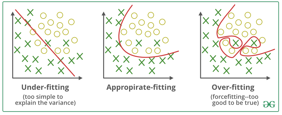
When a model is too simple that it can’t capture the underlying patterns and relationships in the data, then the model can cause an underfitting problem. When a model is too complex and starts to memorize the noise and random fluctuation of the training data instead of learning the underlying structure of the data, then the model can occur overfitting problem and when the model can capture the appropriate patterns of the training data and gives a good performance on training data as well as testing data, then the model can be called as appropriate fit. Our goal is to make the appropriate fitting model.

If Underfitting occurs in the model, then we can take the following steps to overcome the problem.

• Increase the model complexity (add more layers, neurons or use advanced architecture)

• Add more relevant features to the data

• Increase the amount of the data

• If a regularizer is used, then remove that regularizer.

• Change to a different model

Hope, these steps are enough to overcome the problem of underfitting and will get an appropriate fitting model. But if you face an overfitting problem the model gives good performance on training data but poor performance on test data. To overcome the overfitting problem, we have to use a regularization technique that is an addition to the loss function to remove the noise and random fluctuation of the model and get an appropriate fitting model. Today, we will heavily discuss the regularization techniques and hope you will get a deep knowledge about this process.

Let’s go deep. Before deep diving into the sub-topics, let’s get an overview of the topic. They are:

• Introduction

• L1 and L2 Regularization

• Dropout Regularization

• Early Stopping

• Batch Normalization

• Data Augmentation

• Other Regularization Techniques

• Practical Tips and best practices

• Case Studies and Application

• Conclusion

Introduction

Regularizer is a deep learning technique that is used to overcome overfitting and upgrade the performance of the model. Regularization helps to prevent overfitting by adding a penalty to the loss function and it discourages the complex models that fit too closely to the training data. By adding the penalty term to the loss function, the model encourages learning appropriate patterns of the data and performs better on unseen data. Let’s see some benefits of using a regularizer on the overfitted model. 

• It prevents the overfitting problem of the model by adding a penalty term to the loss function.

• It gives better performance on unseen data.

• Some regularization techniques make the model more simpler and interpretable.

• It prevents the model from relying only on one feature of the model and allows the model to learn from more reliable features/ patterns.

• It helps the model to quickly converge.

• It helps the model balance the trade-off of bias-variance. 

It is needed to choose appropriate regularization techniques for specific problems. By choosing and tuning the appropriate regularizer, you can create models that can perform better on unseen data. So, we should understand the depth of each regularizer to apply it perfectly to specific problems. Let’s know the names of the regularizer techniques.

• L1 and L2 regularizer

• Dropout

• Early Stopping

• Data Augmentation

• Batch Normalization

• Elastic Net

• Weight Noise and Activation Noise

• Max Norm Constraints

• Noise injection

There are other regularization techniques and research is ongoing on this topic. Today we will deeply understand the above regularization techniques and how to implement in the problem domain. Let’s go forward.

L1 and L2 Regularization

L1 and L2 are two common techniques used as a regularizer in deep learning models. They prevent overfitting by adding a penalty to the loss function and generalize well on unseen data.

L1 regularizer is also known as Lasso Regularizer. It is used to add a penalty term to the loss function. The penalty term is the sum of the absolute values of all the weights of the model that is multiplied by the regularization parameter(named lambda). Here the lambda is the regularization coefficient that controls the strength of the regularization and it is a hyperparameter that you have to set before training. 

The addition of the penalty to loss function encourages the model to have smaller weights which reduces the model’s complexity and prevents overfitting. It tends to produce sparse weight vectors where many of the weights are zero. This means it forces the model to learn from only a subset of the features of the data. This makes the model perform feature selection, and become more simple and interpretable. 

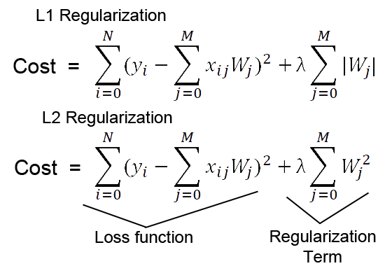
L2 Regularizer is known as Ridge Regularizer. Like the R1 regularizer, It also adds the penalty term to the loss function. Here the penalty term is the sum of the squares of all the weights in the model multiplied by the regularization parameter(lambda). The regularization parameter is a hyperparameter that defines the strength of the regularization in the model. Like R1, it also encourages the model to have smaller weights but unlike R1, it doesn’t force some weights to become zero.

L2 regularizer tends to spread the weight values across all the input features. When all the features are relevant to learn for the model, then L2 regularization can be a better choice than L1 regularizer. Because of producing the small non-zero weights, It can lead to a more stable model. 

The choice of L1 and L2 regularization depends on the problem domain. Let’s see how to implement L1 and L2 regularizers in the model.

Tensorflow

Here ‘kernel_regularizer’ adds L1 or L2 regularization to the weights of the layers and bias_regularizer adds the regularization to the bias. (0.01) is the regularization strength(lambda). You will get the code in Google Colab also.

from tensorflow.keras import regularizers
model = tf.keras.models.Sequential([    # define the L1 or L2 regularizer in kernel and bias regularizer
    tf.keras.layers.Dense(64, kernel_regularizer=regularizers.l1(0.01), bias_regularizer=regularizers.l1(0.01)),
    tf.keras.layers.Dense(64, kernel_regularizer=regularizers.l2(0.01), bias_regularizer=regularizers.l2(0.01)),
    tf.keras.layers.Dense(1)
])

Pytorch

Here L1 and L2 regularization are computed manually. Then the regularization is added to the loss function. L1_lambda or l2_lambda indicates the strength of each regularization.

import torch
import torch.nn as nn
# Define the model
model = nn.Sequential(
    nn.Linear(10, 64),
    nn.ReLU(),
    nn.Linear(64, 1)
)
# Define the loss function
loss_fn = nn.MSELoss()
# L1 regularization
l1_lambda = 0.01
l1_norm = sum(p.abs().sum() for p in model.parameters())
# L2 regularization
l2_lambda = 0.01
l2_norm = sum(p.pow(2.0).sum() for p in model.parameters())
# Add the regularization to the loss
loss = loss_fn(output, target) + l1_lambda * l1_norm + l2_lambda * l2_norm

Hope you have gained a great knowledge about L1 and L2 regularization. Let’s go forward with the DropOut regularization technique.

Dropout Regularization

Dropout is a regularization technique that is used to prevent overfitting by randomly dropping out some of the neurons during training. It reduces the dependence of the network on individual neurons. The motivation behind dropout is to discourage the model from relying too much on a few neurons and force the networks to learn more generalized features. 

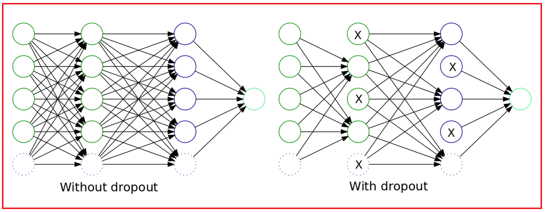
The idea of dropout regularization is simple that is some of the neuron's outputs are randomly ignored or drop out with a certain probability. These dropped-out or ignored neurons will not contribute to the forward pass and also will not participate in the backpropagation.  

It performs several effects in the network which are given below.

• By randomly dropping out some neurons, the network becomes less sensitive to specific weights and makes the model more robust, preventing overfitting and generalizing better on unseen data.

• It reduces the complexity of the model.

• The process of training a model with dropout regularization as like as ensemble method which is known as improved generalization.

• It is computationally efficient and only one hyperparameter is used that indicates the probability of dropping rate.

Let’s understand Dropout probability and Dropout layer for a better understanding of the concept.

Dropout probability indicates the probability of dropout rate in the layer of the model. It is the hyperparameter that is needed to specify before training. If the dropout rate is set to 0.5 that means each neuron of the layer has a 50% chance of being turned off for each training step. 

The dropout layer is a type of layer where dropout can be applied. It can be inserted into fully connected layers, convolution layers or others. It can be applied in the input layer, hidden layers, and so on. During testing, the dropout layer doesn’t deactivate any values.

Hope you get an idea about the concept of the Dropout layer. Let’s see how to implement the dropout regularization technique.

Tensorflow

This is a simple model where a dropout with a 50% probability rate is used in the fully connected layers.

from tensorflow.keras.models import Sequential
from tensorflow.keras.layers import Dense, Dropout
model = Sequential([
    Dense(64, activation='relu', input_shape=(10,)),
    Dropout(0.5),  # Apply dropout with rate of 0.5
    Dense(1, activation='sigmoid')
])

Pytorch

Here we developed a very simple model where a dropout rate of 50% chance is used in the fully connected layers.

import torch
import torch.nn as nn
class Network(nn.Module):
    def __init__(self):
        super(Network, self).__init__()
        self.fc1 = nn.Linear(10, 64)
        self.fc2 = nn.Linear(64, 1)
        # Apply dropout with rate of 0.5
        self.dropout = nn.Dropout(0.5)  
    def forward(self, x):
        x = F.relu(self.fc1(x))
        # perform dropout 
        x = self.dropout(x)
        x = torch.sigmoid(self.fc2(x))
        return x
model = Network()

Hope you have gained a great knowledge about Dropout regularization. Let’s go forward with the Early stopping regularization technique.

Early Stopping

Early stopping is a regularization technique that is used to prevent overfitting by monitoring the validation error during training and stopping the training process at the time of validation error stops to decrease or starts to increase. Easily This method stops the training process when the validation loss function doesn’t decrease or start to increase. 

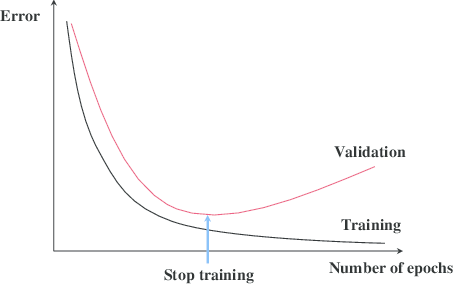
When the training loss is decreasing gradually in a model but the validation loss doesn’t decrease or started to increase gradually, then the model started to learn the noise or fluctuations of the data. So the model gives well performance on training data but poor performance on unseen or validation data, means overfitting problems happen in the model. To solve this problem, Early stopping is used to stop the training process before increasing the validation loss. 

So, The idea of behind early stopping is to monitor the model’s performance on a separate validation dataset during the training process. The training process is stopped when the validation performance starts to degrade. 

Detecting overfitting using the validation set performance and determining the optimal stopping point is essential for the Early Stopping method. Let’s understand the whole process of the Early stopping process below.

• Split the data into three parts(training, validation, and test dataset). A training set is for training, validation is for monitoring the performance of the model, test dataset is for final evaluation.

• Train the model and monitor the validation dataset by tracking the metrics such as accuracy, loss or any other performance measure applicable. 

• Define a criterion for the model when to stop the training process.

• Then keep track of the best model based on the validation metric during training.

• When the stopping criterion is met, stop the training process.

• Load the weights of the best model observed during training.

This is the overall process of the Early stopping regularization method. Hope you can understand the whole process. Let’s go to the implementation part of the Early Stopping regularization technique.

Here we have developed the early stopping process in the model. We have monitored with validation loss and the model will run 3 epochs after degrading the validation loss as patience. We define the early stopping process in callbacks that will be monitored in the training process.

from tensorflow.keras.callbacks import EarlyStopping
# Initialize EarlyStopping callback
early_stopping_callback = EarlyStopping(monitor='val_loss', patience=3)
# Fit model with early stopping
model.fit(X_train, y_train, epochs=100, validation_data=(X_val, y_val), class="dropdown-item",
callbacks=[early_stopping_callback])

Pytorch

Here we have monitored the validation loss function in the training process as early stopping regularization. Another hyperparameter is patience which is used to run the number of epochs after degrading the loss for checking. And also stores the best model based on the validation dataset performance.

import numpy as np
# Parameters
patience = 3
best_loss = np.inf
counter = 0
# Training loop
for epoch in range(100):
    train_loss = train()  
# function to compute train loss
    val_loss = validate()  
# function to compute validation loss
    # Save the model if validation loss decreases
    if val_loss < best_loss:
        best_loss = val_loss
        torch.save(model.state_dict(), 'best_model.pt')
        counter = 0
    
# If validation loss doesn't decrease, increment counter
    else:
        counter += 1
        
# If counter reaches patience, stop training
        if counter >= patience:
            print("Early stopping")
            break
# Load the best model
model.load_state_dict(torch.load('best_model.pt'))

Hope you have gained the overall knowledge about the Early stopping regularization technique. Let’s go forward at the next regularization technique.

Batch Normalization

Batch Normalization is a deep learning technique that is used to improve the stability and performance of neural networks. The idea of batch normalization is to normalize the inputs of each layer to have zero mean and unit variance. Generally, it works by normalizing the activations of each layer(mean of 0 and standard deviation of 1). Input normalization is done before training in the input but batch normalization is done during the training process at each layer and at each training step. 

It solves the internal covariate shift issue in the network. Internal covariate shift describes the distribution of each layer’s input changes during the time by changing the parameters of the previous layers. So, each layer needs to continuously adapt to the new distribution which slows down the training process and makes it hard to converge to the optimal solution. The main cause of it is the updates of the model parameters during training. As the weights of each layer are updated, the inputs of the subsequent layers can shift dramatically and can lead to vanishing gradients or other issues.

Batch Normalization solves the issue by normalizing the inputs to each layer. Batch normalization ensures that the inputs have consistent distribution and allow the network more effectively to learn and generalize from data.

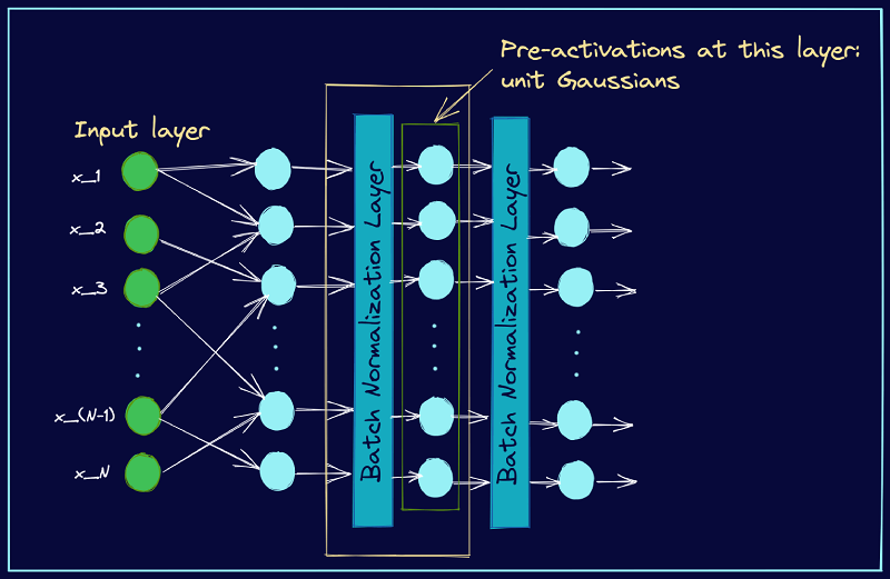
Let’s understand the working process of the Batch normalization is given below.

• For each mini-batch of training data, it calculates the mean and standard deviation of the inputs. 

• Then Normalized the inputs in the mini-batch. The process is to subtract the mean from each input and divide by the square root of the variance plus a small epsilon value.

• Then scale and shift the normalized input by using two new parameters(gamma, beta) that the networks learn. Now we have to multiply the normalized input by Gamma(scale) parameter and add the beta (shift) parameter. 

Batch Normalization has several benefits that are given below.

• The model speeds up learning from the input by normalizing the activations throughout the network. So, it reduces the time to train.

• It allows a higher learning rate in the optimization algorithms.

• It reduces the sensitivity to the initialization of the weights.

• It can be used as a regularization and reduce the need of dropout or other regularization techniques.

• It mitigates the vanishing or exploding gradient problem during the training of the network.

Tensorflow

Here we have defined the batch normalization layer after each hidden layer. 

from tensorflow.keras.models import Sequential
from tensorflow.keras.layers import Dense, BatchNormalization
model = Sequential([
    Dense(64, input_shape=(10,), activation='relu'),
    BatchNormalization(),
    Dense(64, activation='relu'),
    BatchNormalization(),
    Dense(10, activation='softmax')
])

Pytorch

Here we have defined the batch normalization function in bn1 and bn2 and then after each hidden layer batch normalization has been used.

import torch.nn as nn
class Model(nn.Module):
    def __init__(self):
        super(Model, self).__init__()
        self.fc1 = nn.Linear(10, 64)
        self.bn1 = nn.BatchNorm1d(64)
        self.fc2 = nn.Linear(64, 64)
        self.bn2 = nn.BatchNorm1d(64)
        self.fc3 = nn.Linear(64, 10)
    def forward(self, x):
        x = F.relu(self.fc1(x))
        x = self.bn1(x)
        x = F.relu(self.fc2(x))
        x = self.bn2(x)
        x = self.fc3(x)
        return x

Hope You have gained a good understanding and knowledge about Batch Normalization process. Let’s go forward and learn about the Data Augmentation technique.

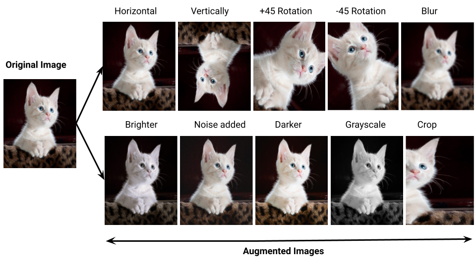
Data Augmentation

Data Augmentation is a technique that is used to increase the amount of the training dataset by creating a variation of the existing dataset. This method can be taken when the original dataset is small or imbalanced. It helps the model to improve the performance and robustness of the deep learning models.

There are several benefits of using the Data Augmentation technique in Deep learning which is given below.

• It increases the number of training data. More amount of data gives more performance of the model. In the small data, a complex neural network starts to memorize the training data instead of learning the underlying patterns in the data. So, an overfitting problem can occur in small data. Data augmentation increases the amount of data and solves the overfitting problem.

• This method increases the diversity of the dataset. This helps the model to learn the main object of the data.

• Because of a more diverse training dataset, the model can’t memorize the training dataset. So, the model starts to understand the underlying patterns in the dataset.

• This method solves the overfitting problem. So it also acts as a regularizer technique.

Data Augmentation techniques can be applied in various data types such as image, text, audio, raw data, and others. Some of the processes of each data type are given below.

Image

• Random Cropping small parts of the images.

• Flipping images horizontally or vertically

• Rotating images in different angles

• Adding random noise in the images

• Zooming in or zooming out of the images and so on.

Text

• Replacing words in a sentence with their synonyms

• Inserting random words in a sentence

• Deleting words from the sentence

• Swapping two words in a sentence and so on

Audio

• Shifting the audio signals forward or backward in time.

• Changing the audio pitch signal with a different tone.

• Adding random noise to the audio signals

• Changing the speed of the audio signal and so on. 

Video

• Cropping a small part of the video frame

• Skipping frames in the video

• Randomly changes brightness, contrast, and others in the video frames

• Flipping the video frame horizontally or vertically and so on.

We have gathered basic knowledge about Data Augmentation. Let’s see how to implement the data augmentation in the model.

Tensorflow

Here we have defined the data augmentation technique, then use that technique in the model. This method can be developed in various ways in TensorFlow. In the data augmentation technique, we use random flipping, random rotation, and random zooming. Other techniques can be taken here.

from tensorflow.keras import layers
import tensorflow as tf
# define data augmentation techniques
  data_augmentation = tf.keras.Sequential([
  layers.RandomFlip("horizontal_and_vertical"),
  layers.RandomRotation(0.2),
  layers.RandomZoom(0.2)
])
model = tf.keras.Sequential([
# apply data augmentation
  data_augmentation,
  layers.Conv2D(16, 3, padding='same', activation='relu'),
  layers.MaxPooling2D(),
  layers.Conv2D(16, 3, padding='same', activation='relu'),
  layers.MaxPooling2D(),
  layers.Flatten(), 
 layers.Dense(10,activation=’softmax’)
])

Pytorch

Here we define the data_augmentation technique in the transform variable. We call this transform technique at the time of loading the dataset from the folder. We have developed a lot of data augmentation techniques such as Horizontal flipping, random rotation, cropping, colorJitter, normalizing input and other techniques also can be taken.

import torch
from torchvision import datasets, transforms
import torch.nn as nn
import torch.nn.functional as F
# Define a transform to augment the data
transform = transforms.Compose([
    transforms.RandomHorizontalFlip(),
    transforms.RandomRotation(10),
    transforms.ColorJitter(brightness=0.1, contrast=0.1, saturation=0.1, hue=0.1),
    transforms.RandomResizedCrop(224, scale=(0.8, 1.0)),
    transforms.ToTensor(),
    transforms.Normalize(mean=[0.485, 0.456, 0.406], std=[0.229, 0.224, 0.225]),
])
# Assuming you have a ImageFolder dataset for your training data
train_dataset = datasets.ImageFolder(root='train_dir', transform=transform)

We have discussed several techniques with respect to regularization techniques. Let’s understand some other regularization techniques that are also used in this criteria to solve the overfitting problem.

Other Regularization Techniques

Elastic Net Regularizer

It is a type of regularization technique that is used to prevent overfitting by adding a penalty term to the loss function. It is a combination of L1 and L2 regularization. L1 helps the model to identify the important features and L2 helps to reduce the impact of the noisy features in the data. The balance of these two regularization techniques makes Elastic net regularization. 

Elastic Net penalty = α * L1 penalty + (1 - α) * L2 penalty

Here alpha is the hyperparameter that controls the balance between L1 and L2. Elastic Net regularizers may overcome the limitations of L1 and L2 regularization. It can be used to overcome the overfitting and make a more stable network. Let’s see how to implement the elastic net regularizer in the following code.

Tensorflow

Here we have defined elastic net regularizer in weights and bias. Kernel_regularizer is for weights and bias_regularizer is for bias.

from tensorflow.keras import regularizers
model = tf.keras.models.Sequential([
    tf.keras.layers.Dense(64, 
                       kernel_regularizer=regularizers.l1_l2(l1=0.01, l2=0.01), # elastic Net(L1 & L2)
                         bias_regularizer=regularizers.l1_l2(l1=0.01, l2=0.01)),
    tf.keras.layers.Dense(1)
])

Pytorch

In the optimizer, we define the weight_decay that indicates the L2 norm and L1 regularization is used in the loss function as the penalty. L1 and L2 both regularization method is used in this network makes the elastic net regularizer.

import torch
import torch.nn as nn
from torch.autograd import Variable
# Assuming you have a model called `model`
model = nn.Linear(10, 1)
# For the optimizer, set weight_decay to be the L2 penalty term
optimizer = torch.optim.SGD(model.parameters(), lr=0.01, weight_decay=0.1)
# For L1 penalty, manually add it to the loss function
l1_lambda = 0.5
l1_norm = sum(p.abs().sum() for p in model.parameters())
# Assuming you have inputs x and targets y
x = Variable(torch.randn(10,10), requires_grad = True)
y = Variable(torch.randn(10,1), requires_grad = True)
# Forward pass
output = model(x)
# Calculate MSE loss
loss = nn.MSELoss()(output, y)
# Add the L1 penalty term to the loss
loss = loss + l1_lambda * l1_norm
# Backward pass and optimization
loss.backward()
optimizer.step()

Weight Noise and Activation Noise

Weight noise and activation noise are the forms of regularization that is used to prevent overfitting in the network. In this process, random noise is added in the weights and activations in the network during training. Weight noise adds noise to the weights of the network and Activation noise adds noise to the output of the neurons. Although it is less useful than other regularization techniques. Let’s see how to implement weight noise and activation noise in the network. 

TensorFlow

from tensorflow.keras import layers
model = tf.keras.models.Sequential([
    layers.Dense(64, activation='relu', input_shape=(10,)),
    layers.GaussianNoise(0.01),
    layers.Dense(1)
])

Pytorch

Here we have added noise to the weights and activation function to prevent overfitting the model and force the model to learn the underlying patterns in the data.

class NoisyLinear(nn.Linear):
    def __init__(self, in_features, out_features, sigma_init=0.017, bias=True):
        super(NoisyLinear, self).__init__(in_features, out_features, bias=bias)
        self.sigma_weight = nn.Parameter(torch.full((out_features, in_features), sigma_init))
        self.register_buffer('epsilon_weight', torch.zeros(out_features, in_features))
        if bias:
            self.sigma_bias = nn.Parameter(torch.full((out_features,), sigma_init))
            self.register_buffer('epsilon_bias', torch.zeros(out_features))
    def forward(self, input):
        self.epsilon_weight.normal_()
        bias = self.bias
        if bias is not None:
            self.epsilon_bias.normal_()
            bias = bias + self.sigma_bias * self.epsilon_bias.data
        return F.linear(input, self.weight + self.sigma_weight * self.epsilon_weight.data, bias)

Max Norm Constraints

Max Norm Constraints define the limit of the total amount of incoming weights to a neuron. It is applied to every neuron of the network. It is a type of weight constraint that limits the maximum value of the L2 norm. It can prevent the weights to become too large and causing overfitting problems in the model. It also improves the performance of the model and works well with the Dropout regularization technique.

Tensorflow

Here in the dense layer, we define the max norm constraints in the kernel constraints so that the weights are limited in the max norm value. 

from tensorflow.keras.constraints import max_norm
model.add(Dense(64, kernel_constraint=max_norm(2.)))

Pytorch 

Here we developed the clip_grad_norm_ function to pass the parameters and max norm arguments to specify the model parameters and the maximum norm value.

from torch.nn.utils import clip_grad_norm_
loss.backward()
clip_grad_norm_(model.parameters(), max_norm=2.)
optimizer.step()

Noise Injection

Noise injection is a type of data augmentation that adds noise to the input data or hidden layers during the training process. Adding noise to the input data or layers, it makes the model more robust and increases the generalization ability of the network. There are some noise injection techniques in deep learning such as Noise injection nodes, Gaussian noise layers, Parametric noise injection, and so on. 

Tensorflow

Here We developed a model and add GaussianNoise in the hidden layer and implement the model so that the model can avoid memorizing the input and avoid the overfitting problems.

from keras.models import Sequential
from keras.layers import Dense
from keras.layers import Activation
from keras.layers import GaussianNoise
# define model
model = Sequential()
model.add(Dense(500, input_dim=2))
model.add(GaussianNoise(0.1)) # Inject Gaussian Noise 
model.add(Activation('relu'))
model.add(Dense(1, activation='sigmoid'))
model.compile(loss='binary_crossentropy', optimizer='adam', metrics=['accuracy'])

Pytorch

You can add a Gaussian noise layer in the model's hidden layers and can implement the model to prevent overfitting. 

import torch.nn as nn
model.add_module("noise", nn.GaussianNoise(0.1))

You can add some random noise to the input data to prevent the overfitting of the model. 

import torch
noise = torch.normal(mean=0.0, std=0.1, size=x.size())
x = x + noise

Practical Tips and Best Practices

The choice of regularization technique depends on the complexity of the model, the size and the quality of the data, and the problem domain. Deep learning is a fact of experiments. It can be beneficial to use a combination of two or more regularization techniques such as L1, drop out at a time, or data augmentation and early stopping or others. The hyperparameter of the regularization techniques (dropout rate, noise level, max_norm rate, penalty coefficients, and so on) can be tuned by cross-validation or other methods to find the optimal values to minimize the validation error. Too much use of regularization can cause underfitting and poor performance on training and validation datasets. So the balance between bias and variance should be maintained. The choice of the regularization technique should be taken by the goal of the model such as accuracy, robustness, interpretability, and so on. Also, we have to consider the data type at the time of choosing the best regularization technique. The best way of choosing the best regularization is to experiment with different regularization techniques in the model and choose the best one that gives the lowest test error and highest accuracy in the validation dataset. Hope you can understand how to use and get the best regularization technique for your model.

Case Studies and Application

Regularization is used in many case studies and applications. Generally in every field (Computer Vision, Audio, Natural Language Processing, Video, and so on) Deep learning uses regularization techniques to improve the performance of unseen data and improve the robustness and interpretability of the model. Actually, regularization is a regular practice in the Deep Learning field. We can use data augmentation in every data type to increase the dataset and improve validation performance. L1 and L2 can be used to remove dependencies of any features. Dropout can reduce the complexity of the model. Early stopping is used to stop the learning process when models start to overfit. Noise injection helps to prevent overfitting of the model. We can use one regularization technique in our model or use two or more regularization techniques at a time in the model to prevent the overfitting and best model. These regularization techniques can be applied in image classification, image segmentation, other computer vision tasks, natural language processing tasks, audio processing tasks, and so on. 

Conclusion

Well. You have understood the importance of regularization techniques in Deep Learning. We have discussed some popular regularization techniques to prevent overfitting and how to implement those in the model. Then we have discussed which regularization technique is needed to choose in specific problem domains and use cases. Hope you have gained an overall knowledge in the field of regularization technique. Actually deep learning is a field of experiment. So experiment more and more to get the best model. On the other hand, research on this topic is ongoing. So new regularization techniques have been developed day by day. You can be updated on these techniques and apply them in your tasks. Thanks for reading the whole tutorial.