Recurrent Neural Networks (RNNs) | Deep Learning

In traditional neural network systems, inputs and outputs are independent of each other. For some situations, previous outputs are required, an example of such cases could be predicting the next word of a sentence. This requires knowledge of the previous words of the existing sentence. Standard neural networks are not very effective in these situations. Here recurrent neural networks can be used instead to solve the problem. Recurrent Neural Networks (RNNs) use internal memory to remember previous outputs. Hence previous information can now be used to influence the current input. 

Recurrent neural networks are a type of neural network which contains internal memory. This feature allows RNNs to remember their previous output, making them suitable for working with sequential data or time series data. They use this memory to take information from prior outputs to affect the next output in the sequence. RNNs use the hidden layer to accomplish this. The hidden state portion of RNN architecture is responsible for memorizing specific information about a sequence. Applications of RNN include working with language modes, such as speech recognition, text classification, automated translation, etc.

RNN vs CNN vs ANN

ANNs (artificial neural networks): Feed-Forward: ANNs are a type of neural network where data travels from input nodes to output nodes through hidden layers in a single direction. Simplicity: Because they lack memory and self-learning capabilities, ANNs are the most basic type of neural network. They are appropriate for jobs that don't require processing in time or sequence. Data Type: ANNs are frequently used to process tabular data, where each input instance is distinct and has no temporal hierarchy. Use: Artificial neural networks (ANNs) are used for a variety of applications, including classification, regression, pattern recognition, and function approximation. Recurrent Neural Networks (RNNs): Recurrent Neural Networks (RNNs) have memory, which enables them to process time-series and sequential input. They keep updated hidden states at each time step, allowing them to keep track of information from earlier inputs. RNNs are particularly effective at handling sequential data, such as time-series data, natural language sentences, and voice. Variable Input Length: RNNs are adaptable for sequential data of varied sizes since they can accept input sequences of varying lengths. Use: Natural Language Processing (NLP) jobs, speech recognition, machine translation, and other sequential data processing tasks all frequently make use of RNNs.  

Convolutional neural networks(CNNs):

Filter-Based Processing: CNNs extract useful patterns and features from spatial data, such as photographs, by combining convolutional layers with filters.

Fixed Input Size: CNNs need fixed-size input, which means that before feeding them with images or spatial data, they must be shrunk to a standard size. Data with a grid-like structure or other spatial data, such as photographs, can be handled by CNNs. CNNs are frequently employed in computer vision tasks such as picture classification, object recognition, image segmentation, and other operations involving examining the visual information in images.

How Recurrent Neural Networks (RNNs) work?

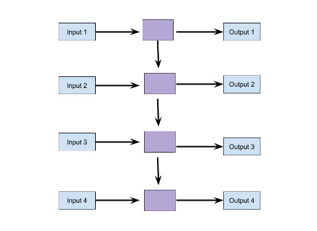
RNN processes data in two directions. Like the feed-forward neural network, it can process input in the forward direction, from initial to final output. In addition to this RNN uses feedback loops. Using this ensures that each input is dependent on the previous input for the decision-making process. 

Let’s consider a simple model with a single neuron. In a traditional neural Network, the input would undergo matrice multiplication with the weight and activation function to produce the output. With RNN the output is used again by feeding it back to itself a specific number of times. This number is called the timestep. It determines how many times output converts to input and gets used for the next matrice multiplication.

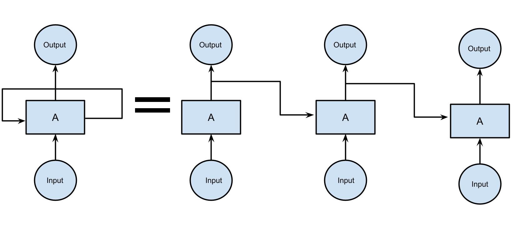
In the diagram above, the middle layer consists of multiple hidden layers, each with its own weights, biases, and activation functions. Each of these layers in the network consists of equal weights and biases. This ensures all the independent variables are now dependent on each other and a single recurrence unit is formed. Now, this single unit can be looped over a specific number of times. 

Overall, this allows the RNN network to take the entire context of a sequence into account when making predictions. For example, if we were to predict the next word in a sentence we can now use the previous words to gain information about the context, making it much more efficient at predicting the next word.

Types of Recurrent Neural Network (RNN)

Vanilla RNNs: There are four types of Vanilla RNNs

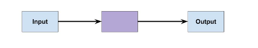
One to One-  These include a single input, a single output, and a feed-forward architecture. Used for simple machine learning problems

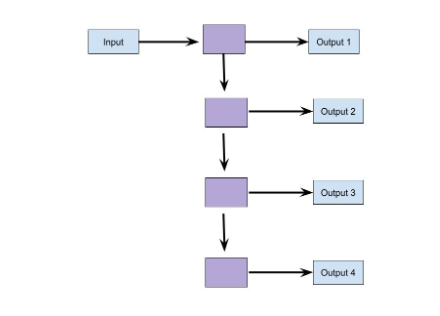
One to Many-  For a single input of fixed size, multiple outputs are provided sequentially. Use cases include image captioning and music generation.

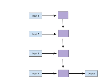
Many to One-  It is used when a single output is required from multiple inputs. For example, in sentiment classification input can be multiple words in a sentence. The output involves providing the likelihood of positive sentiment. In this case, Many to one models can be used for prediction.

Many to Many- Here sequence of inputs is used to produce a sequence of outputs. The number of inputs may be equal to the number of outputs or they may be different. Many to many models are ideal for use cases such as machine translation or name entity recognition where sequential inputs are dependent on each other and context is required for prediction.

Long Short-Term Memory (LSTM) RNNs:

A problem with vanilla RNNs is vanishing gradients where the values of gradient becomes too low during training. LSTM is an extension of RNN which solves this problem.

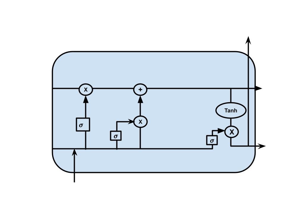
In LSTM, the flow of information is similar to that of RNNs. The difference lies in the cell structure of LSTM. The cell structure consists of various gates and a cell state. The cell state can be considered as the memory of the network. It carries information throughout the processing of the sequence with information being added or removed via the gates. Different neural networks make up the gates of LSTM. These networks determine which information is relevant and which is not during training.

Gates in LSTM contain sigmoid activation functions which enclose values between 0 and 1. This allows the gates to determine which information to keep and which to discard.

LSTM consists of three types of gates:

Forget gate: The main function of the forget gate is to determine which information to discard. Current input and hidden state are passed to a sigmoid function. If the value is close to 0, information is discarded, if it is close to 1, it is kept.

Input Gate: The main purpose of the input gate is to update the cell state. 

First, the current input and hidden state are fed to a sigmoid function to determine which information is relevant or not. To regulate the network, current input, and hidden state also are provided to a tanh function. Finally, the outputs of the two activation functions are multiplied.

Output Gate: The output gate determines what will be the next hidden state. 

Here, the previous hidden state and current input is passed to a sigmoid function. Then the changed cell state is passed to the tanh function. Finally, the output of these two functions is multiplied. In this way what information the hidden state should keep is determined.

With this structure, LSTMs solve the vanishing gradient problem by keeping the gradient steep, which in turn keeps the training relatively short and accuracy high.

Gated Recurrent Unit (GRU) RNNs

GRU has a structure similar to that of LSTM. It is the newer generation of RNNs.

GRU does not use any cell state, rather it uses only hidden states and two gates, reset gate and an update gate to transfer information.

The reset gate has functionalities similar to the input gate and forget gate of LSTM. It decides which information is relevant and which needs to be forgotten

The update gate decides which previous information to forget.

Training RNN

Now we will look at an example of how to train an RNN for text classification. We will code with Tensorflow and Keras and work with Seaborn and Matplotlib for visualization.

Dataset: The dataset we have chosen for this tutorial is the sms spam classification dataset. The dataset can be downloaded from UCI repository. It consists of a collection of texts along with their labels. The categories the texts are divided into are Ham and Spam. Hence we will use this dataset to train our RNN model for text classification of Ham and Spam messages.

After downloading the dataset next we import the necessary libraries. You will get the full code in Google Colab also.

# Importing necessary libraries and modules
# The 'google.colab' module is used for interacting with Google Colab services.
from google.colab import drive
# The 'drive.mount()' function mounts the Google Drive storage to the Colab environment.
drive.mount('/content/drive')
# Importing data manipulation and visualization libraries
# 'numpy' is a powerful library for numerical computing in Python.
import numpy as np
# 'pandas' is a popular library for data manipulation and analysis.
import pandas as pd
# 'matplotlib' is a widely-used library for creating static, interactive, and animated plots in Python.
import matplotlib.pyplot as plt
# 'seaborn' is a data visualization library based on matplotlib, providing an interface for creating attractive statistical .
import seaborn as sns
# It is necessary to visualize the plots without any additional commands.
%matplotlib inline

Here Numpy is a programming language library that supports multi-dimensional arrays and matrices along with a large collection of mathematical functions to operate on these matrices.

Pandas is a python programming library that provides support for data manipulation and analysis. 

Matplotlib is a library for creating animated, static, and interactive visualizations in python language. It is essentially a plotting library.

Seaborn, is a data visualization library which is based on Matplotlib

Next, we read the data which is stored in csv_format using the pandas framework.

ls
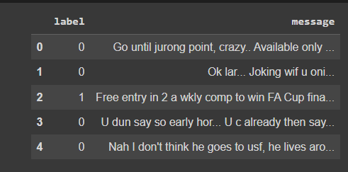
data_frame=pd.read_csv('/content/drive/MyDrive/SMSSpamCollection',sep='\t',names=['label','message']

Here the data is read with column names label and message

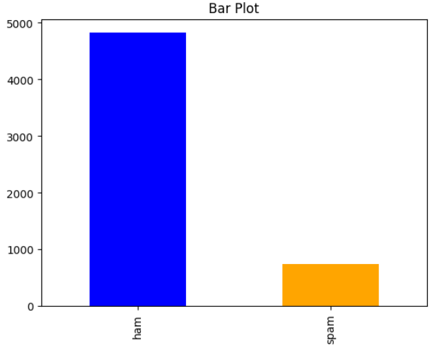
If we want to visualize the data frame with a bar plot, we can do so using the pandas framework again

# The 'sort=True' parameter sorts the counts in descending order.
value_counts_class = pd.value_counts(data_frame["label"], sort=True)
# 'kind='bar'' specifies that we want to create a bar plot.
# The 'color' parameter sets the color of the bars, where ["blue", "orange"] indicates the colors for the bars.
value_counts_class.plot(kind='bar', color=["blue", "orange"])
# Add a title to the bar plot.
plt.title('Bar Plot')
# Display the plot.
plt.show()

The output would give us 

We then provide the labels with numeric values 

# Convert the values in the "label" column of the DataFrame to numerical values.
# are mapped to the values 1 and 0, respectively.
data_frame['label'] = data_frame['label'].map({'spam': 1, 'ham': 0})

Our data frame now looks like this

Now for the training procedure:

We first import tensorflow and keras and import libraries from them

import tensorflow
from tensorflow import keras
#text preprocessing
from keras.preprocessing.text import Tokenizer
from keras.utils import pad_sequences
#model building
from keras.models import Sequential
from keras.layers import Dense
from keras.layers import SimpleRNN
from keras.layers import Flatten
from keras.layers import Dropout
from keras.layers import Embedding
from keras.callbacks import EarlyStopping
# split data into train and test set
from sklearn.model_selection import train_test_split

We can divide this procedure into 3 steps. 

• Data pre-processing

• Model Building

• Splitting of datasets

Preprocessing

First, we need to preprocess the data, this includes using tokenizers and pad sequences. The tokenizer will separate a text into smaller units of tokens. These tokens can be considered as words, characters, or subwords.

We can pad a sentence at the beginning or end using pad_sequence.

Model Building

We can build sequential models using Keras, where we can specify what we want for each layer in the neural network, from input to output.

We also import the simple RNN as the model

We can add other features such as dense layer, dropout, embedding, or flattening along with the imported model.

Splitting dataset

Finally, we import test_train_split from sklearn, which we can use to split our dataset for training and testing.

Having imported the libraries:

We first split the data

# The 'values' attribute converts the Pandas Series to a NumPy array.
X = data_frame['message'].values
# The 'values' attribute converts the Pandas Series to a NumPy array.
y = data_frame['label'].values
# y_train (training target variable), and y_test (testing target variable).
X_train, X_test, y_train, y_test = train_test_split(X, y, test_size=0.20, random_state=42)

We split the data 80:20 here where 80% of the dataset will be used for training and 20% will be used for testing.

We then tokenize the texts and encode them 

# Import the Tokenizer class from the Keras library.
from keras.preprocessing.text import Tokenizer
# Initialize a Tokenizer object.
token = Tokenizer()
# Fit the Tokenizer on the training data (X_train).
# It assigns an index (integer) to each word in the vocabulary for later use in encoding sequences.
token.fit_on_texts(X_train)
# Convert the text data in X_train to sequences of integers using the trained Tokenizer.
# then train_encoded will be [[1, 2], [3, 4, 5]].
train_encoded = token.texts_to_sequences(X_train)
# For example, if X_test contains the text ['hello everyone'], then test_encoded will be [[1]].
test_encoded = token.texts_to_sequences(X_test)

We then pad the data

# Set the maximum length of the sequences. Sequences longer than this will be truncated, and shorter ones will be padded.
maximum_length = 8
# 'padding='post'' means that padding is added at the end of the sequences.
padded_train = pad_sequences(train_encoded, maxlen=maximum_length, padding='post')
# 'padding='post'' means that padding is added at the end of the sequences.
padded_test = pad_sequences(test_encoded, maxlen=maximum_length, padding='post')
# and adding 1 accounts for the reserved index 0 (used for padding).
vocab_size = len(token.word_index) + 1
# Model Definition:
# Create a sequential model, which allows us to build a linear stack of layers.
model = Sequential()
# and 'input_length=maximum_length' specifies the input length for each sequence (padded to the maximum_length).
model.add(Embedding(vocab_size, 24, input_length=maximum_length))
# Add a simple recurrent layer (SimpleRNN) to the model.
model.add(SimpleRNN(24, return_sequences=False))
# The output of this layer will be a probability value between 0 and 1.
model.add(Dense(1, activation='sigmoid'))
# Model Compilation:
# Compile the model with the specified optimizer, loss function, and evaluation metric(s).
model.compile(optimizer='rmsprop', loss='binary_crossentropy', metrics=['accuracy'])

The sequential model is defined by adding an embedding layer before the simple RNN layers and a dense layer after it. The embedding layer is responsible for mapping information from high-dimension to low-dimension space. The dense layer is where every neuron is connected to every other neuron of its preceding layer. The activation function added to the dense layer is sigmoid in this case.

For model compilation the optimizer we use is rmsprop and the loss is binary_crossentropy loss.

Finally, we train the function

# Import the EarlyStopping callback from the Keras library.
from keras.callbacks import EarlyStopping
# Define an EarlyStopping callback with the following settings:
early_stop = EarlyStopping(monitor='val_loss', mode='min', verbose=1, patience=10)
# Fit the model to the training data and validate it on the testing data.
# If the validation loss does not improve for 10 consecutive epochs, training will be stopped early.
model.fit(x=padded_train,
          y=y_train,
          epochs=100,
          validation_data=(padded_test, y_test),
          verbose=1,
          callbacks=[early_stop]
         )

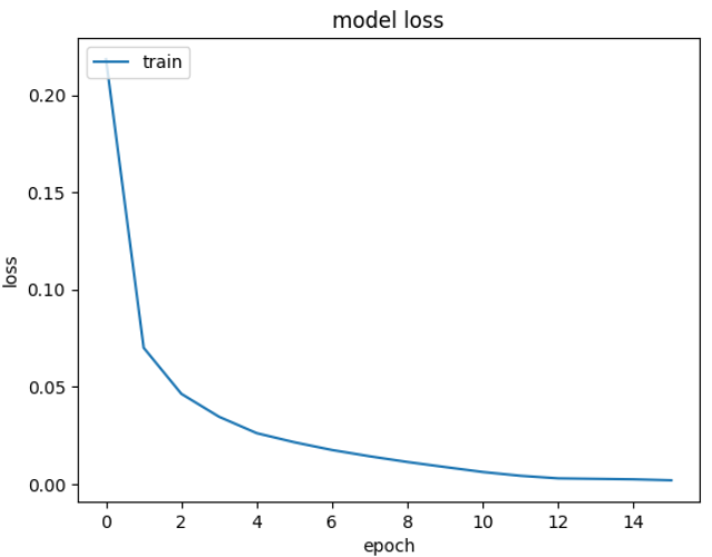
Here we use early stopping which is a regularization technique to avoid overfitting. We train the model for 100 epochs, but due to early stopping training ends at the 16th epoch.

After we plot the training loss the result we found was

# Import the necessary libraries.
from sklearn.metrics import classification_report, confusion_matrix, accuracy_score
import seaborn as sns
import matplotlib.pyplot as plt

# Define a function for displaying the classification report and accuracy score.
def classification_report_display(y_true, y_pred):
   # Print the classification report, which includes precision, recall, F1-score, and support for each class.
   print("Classification Report")
   print(classification_report(y_true, y_pred))
   # Calculate the accuracy score and print it.
   acc_sc = accuracy_score(y_true, y_pred)
   print("Accuracy : " + str(acc_sc))
   # Return the accuracy score for further use if needed.
   return acc_sc
# Define a function for plotting the confusion matrix.
def confusion_matrix_plot(y_true, y_pred):
   # Calculate the confusion matrix using scikit-learn's confusion_matrix function.
   matrix = confusion_matrix(y_true, y_pred)

   # Create a heatmap to visualize the confusion matrix using seaborn.
 
   sns.heatmap(matrix, annot=True, fmt='d', linewidths=.5,
               cmap="Blues", cbar=False)

   # Set the labels for the axes.
   plt.ylabel('True label')
   plt.xlabel('Predicted label')

We then use the classification report and confusion matrix to display the accuracy result on the test set

classification_report_display(y_test, preds)

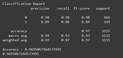
As we can see the accuracy of the model is around 97% which is pretty good. 

confusion_matrix_plot(y_test, preds)

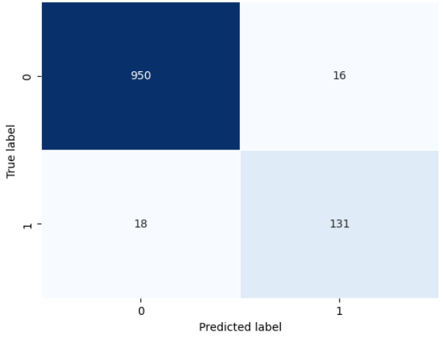
The confusion matrix gives us an understanding of how accurate the model is in predicting the true label of the test set.

Applications of Recurrent Neural Networks (RNNs)

Natural Language Processing: RNN’s are used for text recognition, speech recognition along with many in the natural language processing domain. An example of text recognition has been demonstrated earlier.

Speech Recognition

Speech recognition is the process of identifying words that are spoken aloud and converting them to text.

RNN is better at speech recognition than MLP(Multi layer Perceptron) as it allows variability in the input length. Also since speech recognition involves temporal information, which again is sequential data, RNN is ideal for this situation.

Time series Analysis

Time series data involves observations of a single entity over time. Here LSTM is very effective as it includes long-term memory which allows for more parameters to be learned. Hence, for data that has long-term trends in it, LSTM is the most powerful RNN for these types of situations.

Other Applications:

Other areas where Recurrent Neural Networks can be useful include video tagging, generating image descriptions, face detection, and OCR applications in Image recognition.

Conclusion

RNNs were a giant breakthrough in solving the problem of handling data that needs context for prediction. To need context, you need to have memory, and that is exactly what RNNs provide.

In 2017, Transformer was introduced by Google Brain, which introduced the concept of self-attention. Transformer architecture is increasingly becoming popular in the NLP domain, replacing RNN and LSTM in the process.

RNN is still an important architecture for handling sequential data, it must be learned by anyone trying to understand the process of capturing contextual information in deep learning. One can say RNNs paved the way for transformers to be introduced and recognized.