How to Use LoRA (Low-Rank Adaptation) to Fine-Tune LLMs Efficiently

Fine-tuning big language models (LLMs) including GPT-3, LLaMA, and Mistral means changing every pre-trained model parameter. For most companies, this approach is unworkable nevertheless since it is computationally costly and requires massive storage. GPT-3, for example, has 175 billion trainable parameters, so complete fine-tuning requires great resource-intensity.

By greatly lowering the amount of trainable parameters without sacrificing model performance, LoRA (Low-Rank Adaptation) presents a fast alternative. Unlike adapters, LoRA does not introduce additional inference latency, making it a superior choice for downstream task adaptation.

Challenges of Full Fine-Tuning

Full fine-tuning of large models is highly resource-intensive due to the following reasons:

• Computational Cost: Requires substantial GPU resources.
• Storage Limitations: Storing multiple fine-tuned versions is impractical.
• Scalability Issues: Maintaining and deploying multiple versions increases complexity.

Need for Efficient Adaptation Techniques

Efficient adaptation techniques like LoRA enable organizations to leverage large pre-trained models without excessive computational and storage demands. LoRA provides a cost-effective solution while maintaining or even improving model performance on specific tasks.

Theory and Concept of LoRA

Explanation of LoRA

LoRA operates by freezing the pre-trained model weights and adding trainable low-rank matrices to fit fresh jobs. This approach guarantees good model performance while greatly lowering the amount of trainable parameters.

Importance in Reducing the Number of Trainable Parameters

By using low-rank adaptations, LoRA reduces the amount of parameters to be trained on, therefore enabling effective training with greatly less resources. For implementing big models like GPT-3, this is absolutely vital.

How LoRA Integrates with Existing Architectures

LoRA seamlessly integrates with Transformer architectures by injecting trainable rank-decomposition matrices into each layer without altering the fundamental structure. This ensures compatibility with a wide range of pre-trained models.

Comparison with Other Adaptation Techniques

Other adaptation techniques, such as adapter layers and prefix tuning, introduce additional inference latency due to additional layers. LoRA, however, maintains the original model's inference speed and achieves competitive performance with a fraction of the trainable parameters.

Mathematical Background

Detailed Explanation of Low-Rank Matrix Decomposition

As per inspiration from the paper[1], A neural network typically contains many dense layers with full-rank weight matrices. When adapting these models to specific tasks, we hypothesize that the updates to these weights have a low "intrinsic rank." For a pre-trained weight matrix W₀ ∈ ℝ^{d × k}, LoRA constrains its update ΔW by representing it with a low-rank decomposition.

Wₙ=W₀​+ΔW=W₀​+BA

where B ∈ ℝ^{d × r} and A ∈ ℝ^{r × k}, with r(as per paper experimentation it can be as low as 1 )≪min⁡(d,k)

Let's understand it in simple terms,

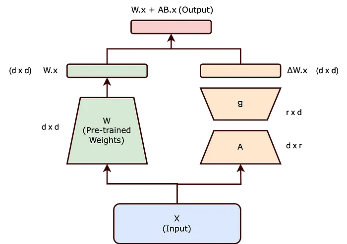
Let's consider a layer with pre-trained weights W and an input x. The output of this layer can be expressed as h = Wx

As mentioned earlier, we will freeze the pre-trained weights W, meaning they will not be updated during backpropagation. Instead, we introduce an additional term ΔW, and all updates will be applied to ΔW.

The new equation becomes:

h=(W+ΔW)x=Wx+ΔWx

Here, W ∈ ℝ^{d × k} and ΔW ∈ ℝ^{d × k}.

Now, we have two options for handling ΔW :

1. Update the entire ΔW matrix, which would require substantial resources and computational power and is same as full-finetuning.
2. Decompose ΔW into two smaller matrices using the LoRA technique.

The first option is essentially the same as the basic method and is resource-intensive. The second option is more efficient: we decompose ΔW into two smaller matrices B and A such that ΔW=BA.

where, B ∈ ℝ^{d × r} A ∈ ℝ^{r × k}, and r is much smaller than both d and k.

Note: An key fact about r is that it increases the number of trainable parameters as we raise r, and therefore training LoRA essentially converges to training the original model.

Updating the matrices A and B uses less memory and processing resources during backpropagation, as they are far smaller than ΔW. The weights have an essentially low rank. Hence, we don't require much information to depict them. We ascertain the rank of the decomposed matrices using the hyperparameter r.

Important notes to remember:

• Matrix A is started with random Gaussian values and matrix B with zeros during training. ΔW=BA therefore initially has zero. α/r scales the term BAx; α is a constant associated with r (usually set to the starting value of r and not tuned). When r changes, this scaling lessens the need to retune hyperparameters.
• Zero extra latency results from merging the modified weights with the base pre-trained weights at inference time.
• We can exchange the modified weights for each use case without reloading the base model if several use cases are fine-tuned on the same base model.

Application of LoRA in Large Language Models

Layers and Weights Targeted

Any subset of weight matrices in a neural network can be used with LoRA to cut the trainable parameter count. Two weight matrices in the MLP module and four in the self-attention module (W_q, Wₖ, Wᵥ, Wₒ) define the Transformer architecture. Though the output dimension is typically cut into attention heads, we consider W_q (or Wₖ, W₅ as a single matrix of dimension d_model ×d_model.[2]

The initial work concentrated on merely freezing the MLP modules (so they are not trained in downstream tasks) both for simplicity and parameter efficiency and adjusting the attention weights (W_q, Wₖ, Wₒ) for downstream tasks.

Excellent results have come from combining weight matrices combined throughout the experimental query (W_q) and value (Wᵥ). Still, separate searches and key weights produce worse performance. Using two weights at once results in a rank r held at 4; fine-tuning single weight metrics at a time results in a rank r kept at 8.

Example Calculation

Step-by-Step Calculation Process of Applying LoRA

Let's consider a hypothetical example to illustrate the process:

1. Original Weight Matrix: W ∈ ℝ^{768 × 768}
2. Rank-Decomposed Matrices: B ∈ ℝ^{768 × 4} and A ∈ ℝ^{4 × 768}
3. Initialization: B is initialized to zeros and A to random values.
4. Update Rule: During training, update only A and B, keeping W frozen.

Hypothetical Example with a Dataset

Suppose we have a model with dimensions d=768 and k=768, and we choose r=4. The original weight matrix W has 589,824 parameters, while the rank-decomposed matrices B and A have only 6,144 parameters combined. This represents a significant reduction.

Implementation of LoRA in Python

Install Dependencies

!pip install datasets
!pip install transformers
!pip install peft
!pip install evaluate

Import Libraries

from datasets import load_dataset, DatasetDict, Dataset
from transformers import (
   AutoTokenizer,
   AutoConfig,
   AutoModelForSequenceClassification,
   DataCollatorWithPadding,
   TrainingArguments,
   Trainer)
from peft import PeftModel, PeftConfig, get_peft_model, LoraConfig
import evaluate
import torch
import numpy as np

Load Dataset

The code loads the SST-2 dataset (Stanford Sentiment Treebank) from the GLUE benchmark using load_dataset("glue", "sst2"), which is commonly used for binary sentiment classification (positive vs. negative). It then calculates the percentage of training samples labeled as "Positive" (label = 1) by summing all 1s in the training labels and dividing by the total number of samples. This helps assess class distribution and potential imbalances in the dataset.

dataset = load_dataset("glue", "sst2")
dataset
# display % of training data with label=1
np.array(dataset['train']['label']).sum()/len(dataset['train']['label'])

Config Model

The code initializes a RoBERTa-based sequence classification model for sentiment analysis. It sets model_checkpoint = 'roberta-base' as the pretrained model and defines label mappings, where 0 corresponds to "Negative" and 1 to "Positive". Using AutoModelForSequenceClassification.from_pretrained(), it loads the RoBERTa model, configuring it for binary classification (num_labels=2) with the provided label mappings (id2label and label2id).

model_checkpoint = 'roberta-base'
# define label maps
id2label = {0: "Negative", 1: "Positive"}
label2id = {"Negative":0, "Positive":1}
# generate classification model from model_checkpoint
model = AutoModelForSequenceClassification.from_pretrained(
   model_checkpoint, num_labels=2, id2label=id2label, label2id=label2id)

Data Preprocessing

The code initializes a tokenizer using AutoTokenizer from a pretrained model checkpoint and ensures it has a padding token by adding [PAD] if missing. It then defines a tokenize_function(examples), which extracts text from the dataset, tokenizes it with left truncation (ensuring important right-side text remains), and limits tokens to 512 max length. The training and validation datasets are tokenized using .map(tokenize_function, batched=True). Finally, a data collator (DataCollatorWithPadding) is created to handle padding dynamically during batch processing.

# create tokenizer
tokenizer = AutoTokenizer.from_pretrained(model_checkpoint, add_prefix_space=True)
# add pad token if none exists
if tokenizer.pad_token is None:
   tokenizer.add_special_tokens({'pad_token': '[PAD]'})
   model.resize_token_embeddings(len(tokenizer))
# create tokenize function
def tokenize_function(examples):
   # extract text
   text = examples["sentence"]
   #tokenize and truncate text
   tokenizer.truncation_side = "left"
   tokenized_inputs = tokenizer(
       text,
       return_tensors="np",
       truncation=True,
       max_length=512
   )
   return tokenized_inputs
# tokenize training and validation datasets
tokenized_dataset = dataset.map(tokenize_function, batched=True)
tokenized_dataset
# create data collator
data_collator = DataCollatorWithPadding(tokenizer=tokenizer)

Evaluation

The code loads the accuracy evaluation metric using evaluate.load("accuracy") and defines a function compute_metrics(p) to calculate accuracy during model evaluation. It extracts predictions and labels from p, applies np.argmax(predictions, axis=1) to get the predicted class labels, and returns the computed accuracy by comparing predictions with actual labels. This function is later used in the Trainer to evaluate model performance.

# import accuracy evaluation metric
accuracy = evaluate.load("accuracy")
# define an evaluation function to pass into trainer later
def compute_metrics(p):
   predictions, labels = p
   predictions = np.argmax(predictions, axis=1)
   return {"accuracy": accuracy.compute(predictions=predictions, references=labels)}

Apply untrained model to text

The code runs an untrained model on a list of example texts to predict sentiment or classification labels. It tokenizes each text using tokenizer.encode(), passes it through the model to compute logits, and then determines the predicted label using torch.argmax(). Finally, it prints the text along with its predicted label from the id2label mapping.

# define list of examples
text_list = ["a feel-good picture in the best sense of the term .", "resourceful and ingenious entertainment .", "it 's just incredibly dull .", "the movie 's biggest offense is its complete and utter lack of tension .",
            "impresses you with its open-endedness and surprises .", "unless you are in dire need of a diesel fix , there is no real reason to see it ."]
print("Untrained model predictions:")
print("----------------------------")
for text in text_list:
   # tokenize text
   inputs = tokenizer.encode(text, return_tensors="pt")
   # compute logits
   logits = model(inputs).logits
   # convert logits to label
   predictions = torch.argmax(logits)
   print(text + " - " + id2label[predictions.tolist()])

Output:

Untrained model predictions:
----------------------------
a feel-good picture in the best sense of the term . - Negative
resourceful and ingenious entertainment . - Negative
it 's just incredibly dull . - Negative
the movie 's biggest offense is its complete and utter lack of tension . - Negative
impresses you with its open-endedness and surprises . - Negative
unless you are in dire need of a diesel fix , there is no real reason to see it . - Negative

Train the model

The code defines a LoRA (Low-Rank Adaptation) configuration for fine-tuning a transformer model efficiently. It sets key parameters like r=4 (low-rank decomposition), lora_alpha=32 (scaling factor), and lora_dropout=0.01 (dropout to prevent overfitting). The target_modules=['query'] ensures only the query projection layer is fine-tuned, keeping the rest frozen. This approach reduces trainable parameters while maintaining performance in sequence classification (SEQ_CLS) tasks.

peft_config = LoraConfig(task_type="SEQ_CLS",
                       r=4,
                       lora_alpha=32,
                       lora_dropout=0.01,
                       target_modules = ['query'])
peft_config

Output:

LoraConfig(task_type='SEQ_CLS', peft_type=<PeftType.LORA: 'LORA'>, auto_mapping=None, base_model_name_or_path=None, revision=None, inference_mode=False, r=4, target_modules={'query'}, exclude_modules=None, lora_alpha=32, lora_dropout=0.01, fan_in_fan_out=False, bias='none', use_rslora=False, modules_to_save=None, init_lora_weights=True, layers_to_transform=None, layers_pattern=None, rank_pattern={}, alpha_pattern={}, megatron_config=None, megatron_core='megatron.core', loftq_config={}, eva_config=None, use_dora=False, layer_replication=None, runtime_config=LoraRuntimeConfig(ephemeral_gpu_offload=False), lora_bias=False)
model = get_peft_model(model, peft_config)
model.print_trainable_parameters()

Output:

trainable params: 665,858 || all params: 125,313,028 || trainable%: 0.5314

Training a Text Classification Model with Transformers' Trainer API

The code sets up and trains a text classification model using the Trainer API from the transformers library. It first defines hyperparameters like learning rate, batch size, and the number of training epochs. Then, it configures training arguments, specifying settings such as the output directory, learning rate, batch sizes for training and evaluation, weight decay, and strategies for evaluation and model saving. Next, it initializes a Trainer object with the model, training arguments, tokenized datasets, tokenizer, data collator, and evaluation metric function. The model is then trained using trainer.train(). However, the code redundantly reinitializes the Trainer with the same settings and retrains the model again, which is unnecessary since the first training call already trains the model.

# hyperparameters
lr = 1e-3
batch_size = 16
num_epochs = 5
# define training arguments
training_args = TrainingArguments(
   output_dir= model_checkpoint + "-lora-text-classification",
   learning_rate=lr,
   per_device_train_batch_size=batch_size,
   per_device_eval_batch_size=batch_size,
   num_train_epochs=num_epochs,
   weight_decay=0.01,
   evaluation_strategy="epoch",
   save_strategy="epoch",
   load_best_model_at_end=True,
)
# creater trainer object
trainer = Trainer(
   model=model,
   args=training_args,
   train_dataset=tokenized_dataset["train"],
   eval_dataset=tokenized_dataset["validation"],
   tokenizer=tokenizer,
   data_collator=data_collator,
   compute_metrics=compute_metrics,
)
# train model
trainer.train()
# creater trainer object
trainer = Trainer(
   model=model,
   args=training_args,
   train_dataset=tokenized_dataset["train"],
   eval_dataset=tokenized_dataset["validation"],
   tokenizer=tokenizer,
   data_collator=data_collator,
   compute_metrics=compute_metrics,
)
# train model
trainer.train()

Output:

Generate prediction

The code moves the trained model to the CPU, then iterates through a list of texts, tokenizes each text, gets model predictions, and prints the predicted label.

model.to('cpu')
print("Trained model predictions:")
print("--------------------------")
for text in text_list:
   inputs = tokenizer.encode(text, return_tensors="pt").to("cpu")
   logits = model(inputs).logits
   predictions = torch.max(logits,1).indices
   print(text + " - " + id2label[predictions.tolist()[0]])

Output:

Trained model predictions:
--------------------------
a feel-good picture in the best sense of the term . - Positive
resourceful and ingenious entertainment . - Positive
it 's just incredibly dull . - Negative
the movie 's biggest offense is its complete and utter lack of tension . - Negative
impresses you with its open-endedness and surprises . - Positive
unless you are in dire need of a diesel fix , there is no real reason to see it . - Negative

Advantages of LoRA

1. Reduced Trainable Parameters: Achieves a 99% reduction compared to full fine-tuning.
2. Lower Computational Cost: Requires significantly fewer resources.
3. Zero Additional Latency: The adapted weights can be merged with the base model at inference time.
4. Scalability: Enables quick adaptation to multiple downstream tasks.
5. Flexibility: Can be applied to different transformer layers based on computational budgets.

Conclusion

LoRA is a game-changer in efficient model fine-tuning, enabling the adaptation of large language models with minimal computational overhead. By leveraging low-rank adaptations, LoRA achieves performance comparable to full fine-tuning while requiring significantly fewer resources. Its ability to integrate seamlessly with existing architectures and maintain inference speed makes it an ideal choice for deploying large-scale AI applications.

References

[1] https://arxiv.org/abs/2012.13255

[2] https://arxiv.org/abs/2106.09685