Generative modeling using Variational AutoEncoders | Generative AI

Written by- AionlinecourseGenerative AI Tutorials

Introduction

Algorithms used in generative modeling in AI and machine learning produce fresh data in addition to classifying and predicting it. By examining the underlying structure of data, Variational AutoEncoders (VAEs) are a potent tool that fosters innovation in artificial intelligence. With the help of neural networks and probabilistic modeling concepts, VAEs are able to learn the distribution of potential latent representations. The architecture, training, and learning processes of VAEs are all covered in this tutorial. A unique method for producing realistic text, graphics, and other data formats is provided by VAEs.

Importance of Variational AutoEncoders (VAEs)

Variational autoencoders (VAEs) are essential for probabilistic generative modelling and unsupervised learning. For applications including picture synthesis, anomaly detection, data imputation, and drug discovery, they produce a wide range of realistic samples. Virtual Analogue Engines (VAEs) are vital in many sectors because they extract important properties from data structures and use them to create new data points that are much like the originals.

Understanding Autoencoders in VAEs

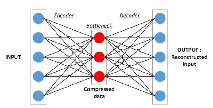
Autoencoders are techniques for unsupervised learning that acquire compressed representations of input data without the need for explicit labels. Their goal is to find linkages, structures, or hidden patterns in the data by itself. An encoder network maps the input data to a lower-dimensional latent space, while a decoder network reconstructs the original data from the latent representation. This is how autoencoders function. Together, the encoder and decoder are trained to reduce reconstruction error and extract the most important information.

Key Components of VAEs

Encoder: Within VAEs, the encoder serves as a translator, interpreting the input data and capturing all of its nuances and specifics. It exposes possible interpretations inside the latent space by mapping the data point to a probability distribution that crosses the space. A more thorough comprehension and portrayal of cultural nuances and implications are made possible by this procedure.

Latent Space: Within VAEs, the latent space is a smooth and seamless landscape for exploration. It is a lower-dimensional representation that captures the essential components of the input data. Because of its continuous architecture, interpolation and imaginative trips between data points are possible. Points from the learned distribution are sampled in order to navigate this concealed domain; these samples, when sent through the decoder network, can reveal new and distinct data points.

Decoder: In the original data space, the Decoder is a machine that can translate ideas from abstract to concrete forms. To ensure the integrity of the input data is restored, it maps a point in the latent space back to the original data space. By producing fresh data points that mimic the original input and reduce reconstruction error, the decoder adds novelty while maintaining the original input's qualities.

Implementation of Variational AutoEncoders (VAEs)

Step 1: Import libraries

import numpy as np
import matplotlib.pyplot as plt
from scipy.stats import norm
import tensorflow as tf
import tensorflow.keras.backend as K
from tensorflow.keras import (
    layers,
    models,
    datasets,
    callbacks,
    losses,
    optimizers,
    metrics,
)
    batch = dataset.take(1).get_single_element()
    if isinstance(batch, tuple):
        batch = batch[0]
    return batch.numpy()
def display(
    images, n=10, size=(20, 3), cmap="gray_r", as_type="float32", save_to=None
):
    """
    Displays n random images from each one of the supplied arrays.
    """
    if images.max() > 1.0:
        images = images / 255.0
    elif images.min() < 0.0:
        images = (images + 1.0) / 2.0
    plt.figure(figsize=size)
    for i in range(n):
        _ = plt.subplot(1, n, i + 1)
        plt.imshow(images[i].astype(as_type), cmap=cmap)
        plt.axis("off")
    if save_to:
        plt.savefig(save_to)
        print(f"\nSaved to {save_to}")
    plt.show()

def sample_batch(dataset):

Step 2: Data Preparation

(x_train, y_train), (x_test, y_test) = datasets.fashion_mnist.load_data()

Output results:

Downloading data from https://storage.googleapis.com/tensorflow/tf-keras-datasets/train-labels-idx1-ubyte.gz
29515/29515 [==============================] - 0s 0us/step
Downloading data from https://storage.googleapis.com/tensorflow/tf-keras-datasets/train-images-idx3-ubyte.gz
26421880/26421880 [==============================] - 0s 0us/step
Downloading data from https://storage.googleapis.com/tensorflow/tf-keras-datasets/t10k-labels-idx1-ubyte.gz
5148/5148 [==============================] - 0s 0us/step
Downloading data from https://storage.googleapis.com/tensorflow/tf-keras-datasets/t10k-images-idx3-ubyte.gz
4422102/4422102 [==============================] - 0s 0us/step

Step 3: Data Preprocessing

def preprocess(imgs):
    """
    Normalize and reshape the images
    """
    imgs = imgs.astype("float32") / 255.0
    imgs = np.pad(imgs, ((0, 0), (2, 2), (2, 2)), constant_values=0.0)
    imgs = np.expand_dims(imgs, -1)
    return imgs
x_train = preprocess(x_train)
x_test = preprocess(x_test)

Step 4: Designing and Building Variational Autoencoder

#Sampling Layerclass Sampling(layers.Layer):
    #We create a new layer by subclassing the keras base Layer
    def call(self, inputs):
        #
        z_mean, z_log_var = inputs
        batch = tf.shape(z_mean)[0]
        dim = tf.shape(z_mean)[1]
        epsilon = K.random_normal(shape=(batch, dim))
        return z_mean + tf.exp(0.5 * z_log_var) * epsilon
# Encoder
image_size = 32
embed_dim = 2
encoder_input = layers.Input(
    shape=(image_size, image_size, 1), name="encoder_input"
)
x = layers.Conv2D(32, (3, 3), strides=2, activation="relu", padding="same")(
    encoder_input
)
x = layers.Conv2D(64, (3, 3), strides=2, activation="relu", padding="same")(x)
x = layers.Conv2D(128, (3, 3), strides=2, activation="relu", padding="same")(x)
shape_before_flattening = K.int_shape(x)[1:]  # the decoder will need this!
x = layers.Flatten()(x)

z_mean = layers.Dense(embed_dim, name="z_mean")(x)
z_log_var = layers.Dense(embed_dim, name="z_log_var")(x)

z = Sampling()([z_mean, z_log_var])

encoder = models.Model(encoder_input, [z_mean, z_log_var, z], name="encoder")
encoder.summary()

Output results:

Model: "encoder"
__________________________________________________________________________________________________
 Layer (type)                Output Shape                 Param #   Connected to                  
==================================================================================================
 encoder_input (InputLayer)  [(None, 32, 32, 1)]          0         []                            
                                                                                                  
 conv2d (Conv2D)             (None, 16, 16, 32)           320       ['encoder_input[0][0]']       
                                                                                                  
 conv2d_1 (Conv2D)           (None, 8, 8, 64)             18496     ['conv2d[0][0]']              
                                                                                                  
 conv2d_2 (Conv2D)           (None, 4, 4, 128)            73856     ['conv2d_1[0][0]']            
                                                                                                  
 flatten (Flatten)           (None, 2048)                 0         ['conv2d_2[0][0]']            
                                                                                                  
 z_mean (Dense)              (None, 2)                    4098      ['flatten[0][0]']             
                                                                                                  
 z_log_var (Dense)           (None, 2)                    4098      ['flatten[0][0]']             
                                                                                                  
 sampling (Sampling)         (None, 2)                    0         ['z_mean[0][0]',              
                                                                     'z_log_var[0][0]']           
                                                                                                  
==================================================================================================
Total params: 100868 (394.02 KB)
Trainable params: 100868 (394.02 KB)
Non-trainable params: 0 (0.00 Byte)
__________________________________________________________________________________________________

# Decoder
decoder_input = layers.Input(shape=(embed_dim,), name="decoder_input")
x = layers.Dense(np.prod(shape_before_flattening))(decoder_input)
x = layers.Reshape(shape_before_flattening)(x)
x = layers.Conv2DTranspose(
    128, (3, 3), strides=2, activation="relu", padding="same"
)(x)
x = layers.Conv2DTranspose(
    64, (3, 3), strides=2, activation="relu", padding="same"
)(x)
x = layers.Conv2DTranspose(
    32, (3, 3), strides=2, activation="relu", padding="same"
)(x)
decoder_output = layers.Conv2D(
    1,
    (3, 3),
    strides=1,
    activation="sigmoid",
    padding="same",
    name="decoder_output",
)(x)
decoder = models.Model(decoder_input, decoder_output)
decoder.summary()

Output results:

Model: "model"
_________________________________________________________________
 Layer (type)                Output Shape              Param #   
=================================================================
 decoder_input (InputLayer)  [(None, 2)]               0         
                                                                 
 dense (Dense)               (None, 2048)              6144      
                                                                 
 reshape (Reshape)           (None, 4, 4, 128)         0         
                                                                 
 conv2d_transpose (Conv2DTr  (None, 8, 8, 128)         147584    
 anspose)                                                        
                                                                 
 conv2d_transpose_1 (Conv2D  (None, 16, 16, 64)        73792     
 Transpose)                                                      
                                                                 
 conv2d_transpose_2 (Conv2D  (None, 32, 32, 32)        18464     
 Transpose)                                                      
                                                                 
 decoder_output (Conv2D)     (None, 32, 32, 1)         289       
                                                                 
=================================================================
Total params: 246273 (962.00 KB)
Trainable params: 246273 (962.00 KB)
Non-trainable params: 0 (0.00 Byte)
_________________________________________________________________

Step 5: Lets Train our Variational Autoencoder

class VAE(models.Model):
    def __init__(self, encoder, decoder, **kwargs):
        super(VAE, self).__init__(**kwargs)
        self.encoder = encoder
        self.decoder = decoder
        self.total_loss_tracker = metrics.Mean(name="total_loss")
        self.reconstruction_loss_tracker = metrics.Mean(
            name="reconstruction_loss"
        )
        self.kl_loss_tracker = metrics.Mean(name="kl_loss")
    @property
    def metrics(self):
        return [
            self.total_loss_tracker,
            self.reconstruction_loss_tracker,
            self.kl_loss_tracker,
        ]
    def call(self, inputs):
        """Call the model on a particular input."""
        z_mean, z_log_var, z = encoder(inputs)
        reconstruction = decoder(z)
        return z_mean, z_log_var, reconstruction
    def train_step(self, data):
        """Step run during training."""
        with tf.GradientTape() as tape:

            z_mean, z_log_var, reconstruction = self(data)
            beta = 500
            reconstruction_loss = tf.reduce_mean(
                beta
                * losses.binary_crossentropy(
                    data, reconstruction, axis=(1, 2, 3)
                )
            )
            kl_loss = tf.reduce_mean(
                tf.reduce_sum(
                    -0.5
                    * (1 + z_log_var - tf.square(z_mean) - tf.exp(z_log_var)),
                    axis=1,
                )
            )
            total_loss = reconstruction_loss + kl_loss
        grads = tape.gradient(total_loss, self.trainable_weights)
        self.optimizer.apply_gradients(zip(grads, self.trainable_weights))
        self.total_loss_tracker.update_state(total_loss)
        self.reconstruction_loss_tracker.update_state(reconstruction_loss)
        self.kl_loss_tracker.update_state(kl_loss)
        return {m.name: m.result() for m in self.metrics}
    def test_step(self, data):
        """Step run during validation."""
        if isinstance(data, tuple):
            data = data[0]
        z_mean, z_log_var, reconstruction = self(data)
        beta = 500
        reconstruction_loss = tf.reduce_mean(
            beta
            * losses.binary_crossentropy(data, reconstruction, axis=(1, 2, 3))
        )
        kl_loss = tf.reduce_mean(
            tf.reduce_sum(
                -0.5 * (1 + z_log_var - tf.square(z_mean) - tf.exp(z_log_var)),
                axis=1,
            )
        )
        total_loss = reconstruction_loss + kl_loss
        return {
            "loss": total_loss,
            "reconstruction_loss": reconstruction_loss,
            "kl_loss": kl_loss,
        }

vae = VAE(encoder, decoder)

Step 6: Starting Training

# Compile the variational autoencoder
optimizer = optimizers.Adam(learning_rate=0.0005)
vae.compile(optimizer=optimizer)
model_checkpoint_callback = callbacks.ModelCheckpoint(
    filepath="./checkpoint",
    save_weights_only=False,
    save_freq="epoch",
    monitor="loss",
    mode="min",
    save_best_only=True,
    verbose=0,
)
tensorboard_callback = callbacks.TensorBoard(log_dir="./logs")

vae.fit(
    x_train,
    epochs=5,
    batch_size=50,
    shuffle=True,
    validation_data=(x_test, x_test),
    callbacks=[model_checkpoint_callback, tensorboard_callback],
)

Output results:

Epoch 1/5
1195/1200 [============================>.] - ETA: 0s - total_loss: 150.8727 - reconstruction_loss: 146.2451 - kl_loss: 4.6275WARNING:tensorflow:Can save best model only with loss available, skipping.
1200/1200 [==============================] - 17s 8ms/step - total_loss: 150.8177 - reconstruction_loss: 146.1882 - kl_loss: 4.6294 - val_loss: 136.6184 - val_reconstruction_loss: 131.4518 - val_kl_loss: 5.1666
Epoch 2/5
1197/1200 [============================>.] - ETA: 0s - total_loss: 134.7354 - reconstruction_loss: 129.7034 - kl_loss: 5.0320WARNING:tensorflow:Can save best model only with loss available, skipping.
1200/1200 [==============================] - 8s 7ms/step - total_loss: 134.7361 - reconstruction_loss: 129.7041 - kl_loss: 5.0320 - val_loss: 134.5743 - val_reconstruction_loss: 129.4605 - val_kl_loss: 5.1138
Epoch 3/5
1200/1200 [==============================] - ETA: 0s - total_loss: 133.2709 - reconstruction_loss: 128.1776 - kl_loss: 5.0934WARNING:tensorflow:Can save best model only with loss available, skipping.
1200/1200 [==============================] - 8s 7ms/step - total_loss: 133.2709 - reconstruction_loss: 128.1776 - kl_loss: 5.0934 - val_loss: 133.8215 - val_reconstruction_loss: 128.5919 - val_kl_loss: 5.2296
Epoch 4/5
1198/1200 [============================>.] - ETA: 0s - total_loss: 132.4913 - reconstruction_loss: 127.3487 - kl_loss: 5.1428WARNING:tensorflow:Can save best model only with loss available, skipping.
1200/1200 [==============================] - 9s 7ms/step - total_loss: 132.4916 - reconstruction_loss: 127.3490 - kl_loss: 5.1428 - val_loss: 132.6691 - val_reconstruction_loss: 127.3441 - val_kl_loss: 5.3251
Epoch 5/5
1197/1200 [============================>.] - ETA: 0s - total_loss: 131.9378 - reconstruction_loss: 126.7507 - kl_loss: 5.1871WARNING:tensorflow:Can save best model only with loss available, skipping.
1200/1200 [==============================] - 8s 7ms/step - total_loss: 131.9424 - reconstruction_loss: 126.7551 - kl_loss: 5.1873 - val_loss: 132.3715 - val_reconstruction_loss: 126.9836 - val_kl_loss: 5.3879
<keras.src.callbacks.History at 0x79797b6c80a0>

Step 7: Saving Trained Checkpoints

# Save the final models
vae.save("./models/vae")
encoder.save("./models/encoder")
decoder.save("./models/decoder")

Step 8: Lets try to reconstruct using our trained variational autoencoder

n_to_predict = 5000
example_images = x_test[:n_to_predict]
example_labels = y_test[:n_to_predict]
z_mean, z_log_var, reconstructions = vae.predict(example_images)
print("Example real clothing items")
# display(example_images)
print("Reconstructions")

Output results:

157/157 [==============================] - 1s 5ms/step
Example real clothing items
Reconstructions

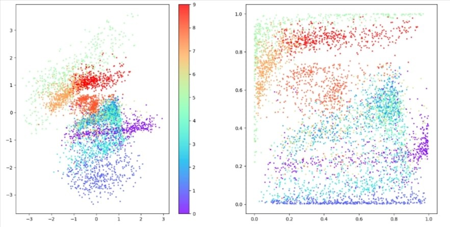
Step 9: Lets visualize Latent Space

z_mean, z_var, z = encoder.predict(example_images)
p = norm.cdf(z)

Output results:

157/157 [==============================] - 0s 2ms/step

figsize = 8
fig = plt.figure(figsize=(figsize * 2, figsize))
ax = fig.add_subplot(1, 2, 1)
plot_1 = ax.scatter(
    z[:, 0], z[:, 1], cmap="rainbow", c=example_labels, alpha=0.8, s=3
)
plt.colorbar(plot_1)
ax = fig.add_subplot(1, 2, 2)
plot_2 = ax.scatter(
    p[:, 0], p[:, 1], cmap="rainbow", c=example_labels, alpha=0.8, s=3
)
plt.show()

Output results:

Conclusion

Variational AutoEncoders (VAEs) are used in AI and machine learning to recreate images, as this lesson illustrates. Using TensorFlow and Keras, the VAE generates points in a latent space, reconstructs images, and extracts meaningful representations. The trained VAE improved machine learning and artificial intelligence by correctly reconstructing images.

Previous Next